ALEX Intelligence Expired Property Seller Model · Version 14.462 · Comparables identified by the system
Prepared for —
· Prepared by Diane Hart Alexander, MBA, MHA, Designated Broker
This is a comparable-sales opinion of value, not a certified
appraisal. It is not a mortgage or lending document. It draws on ABOR MLS listing and sale records, delivered through secure APIs,
on county appraisal district records, and many other secure API datasets. Tax values come from the local County Appraisal District (CAD) if available; if not, from a secure API. ALEX’s adjustment engine does the calculations.
Subject to Diane’s
refinements.
Privileged & Confidential
For use by ALEX Agents and Clients only.
Sharing this report or its information with any third party without
ALEX’s express written consent is prohibited and subjects the
disclosing party to legal action.
It combines the ALEX Model and the ALEX Slotting Tool. The valuation model reads the comparable sales. The slotting tool sets the price just under a common search price and the nearest competing listing, and under the price the market already declined.
Three figures, one story. The valuation, $1,065,936,
is what the comparable sales say this home is worth, net of concessions. The sale price,
$1,067,500, is that value with the buyer’s closing costs and repairs
sellers here customarily pay added back. The recommended list price is where to ask.
If you want to discuss the recommended list price,
contact Diane (your agent).
The listing that did not sell
Date
List price
Reduction
Original list price
08/06/2026
$1,245,000
—
Last list price
08/24/2026
$1,195,000
−$50,000 (4.0%)
Total reductions
−$50,000 (4.0%)
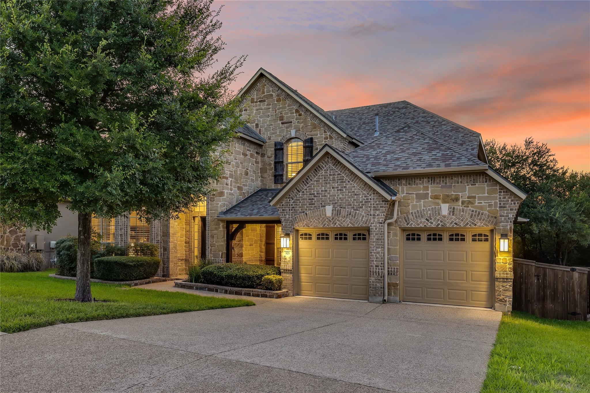
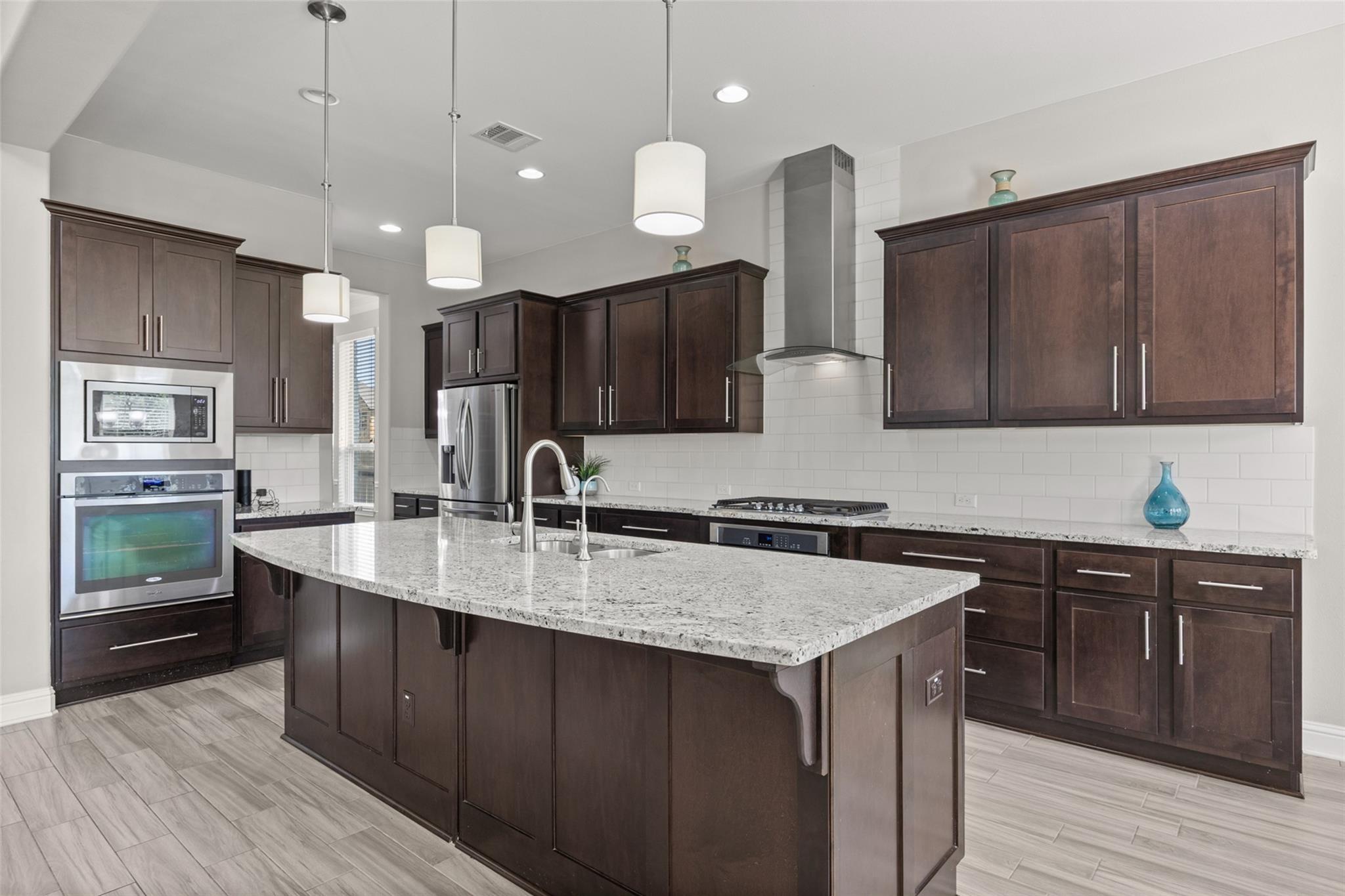
Water view
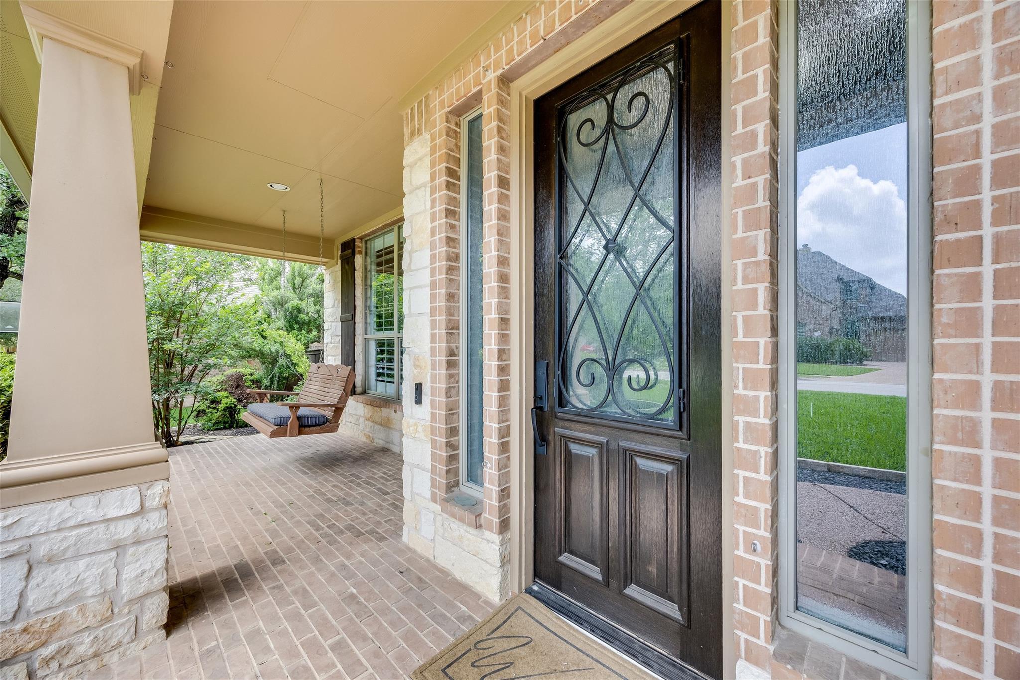
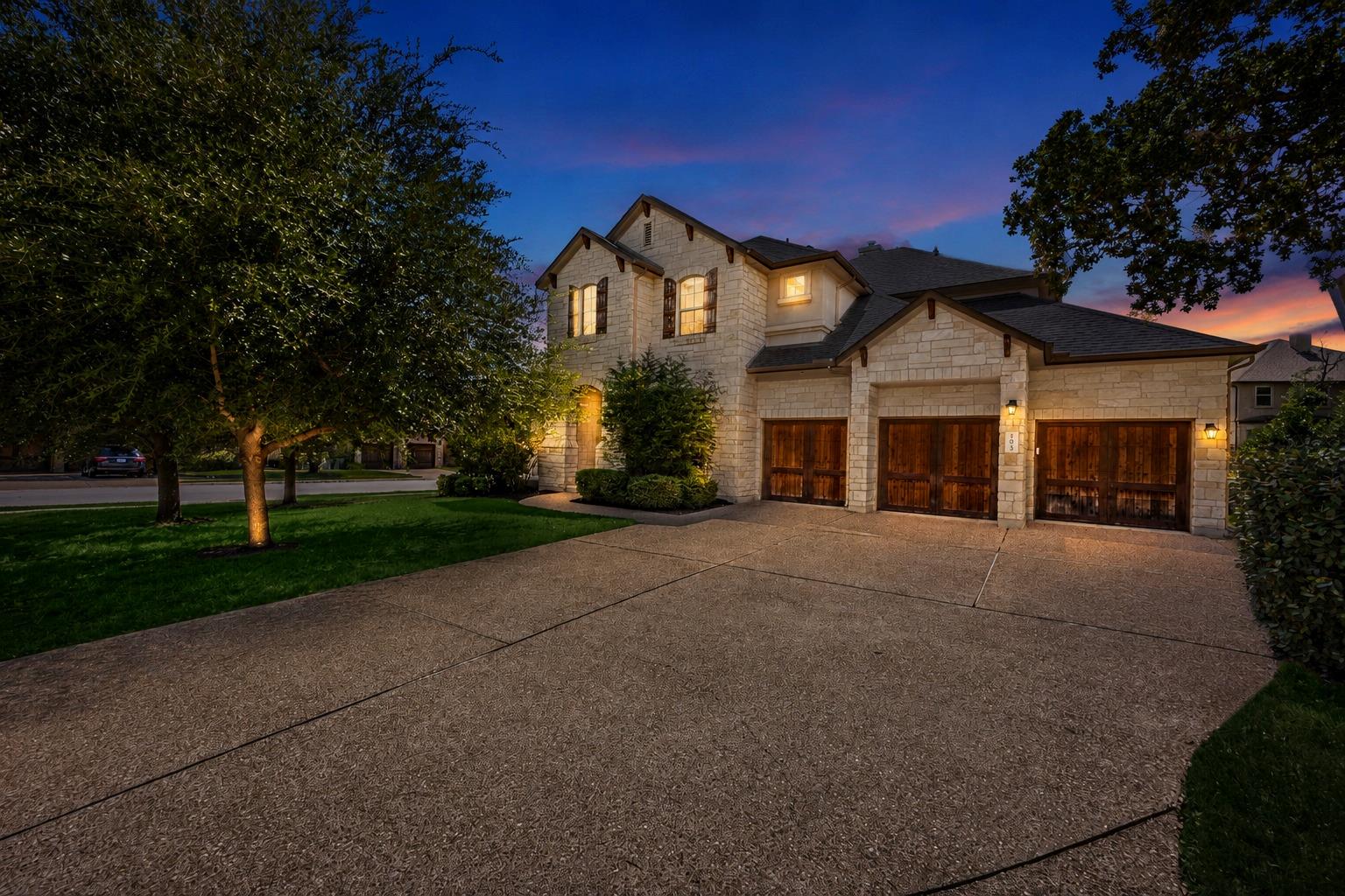
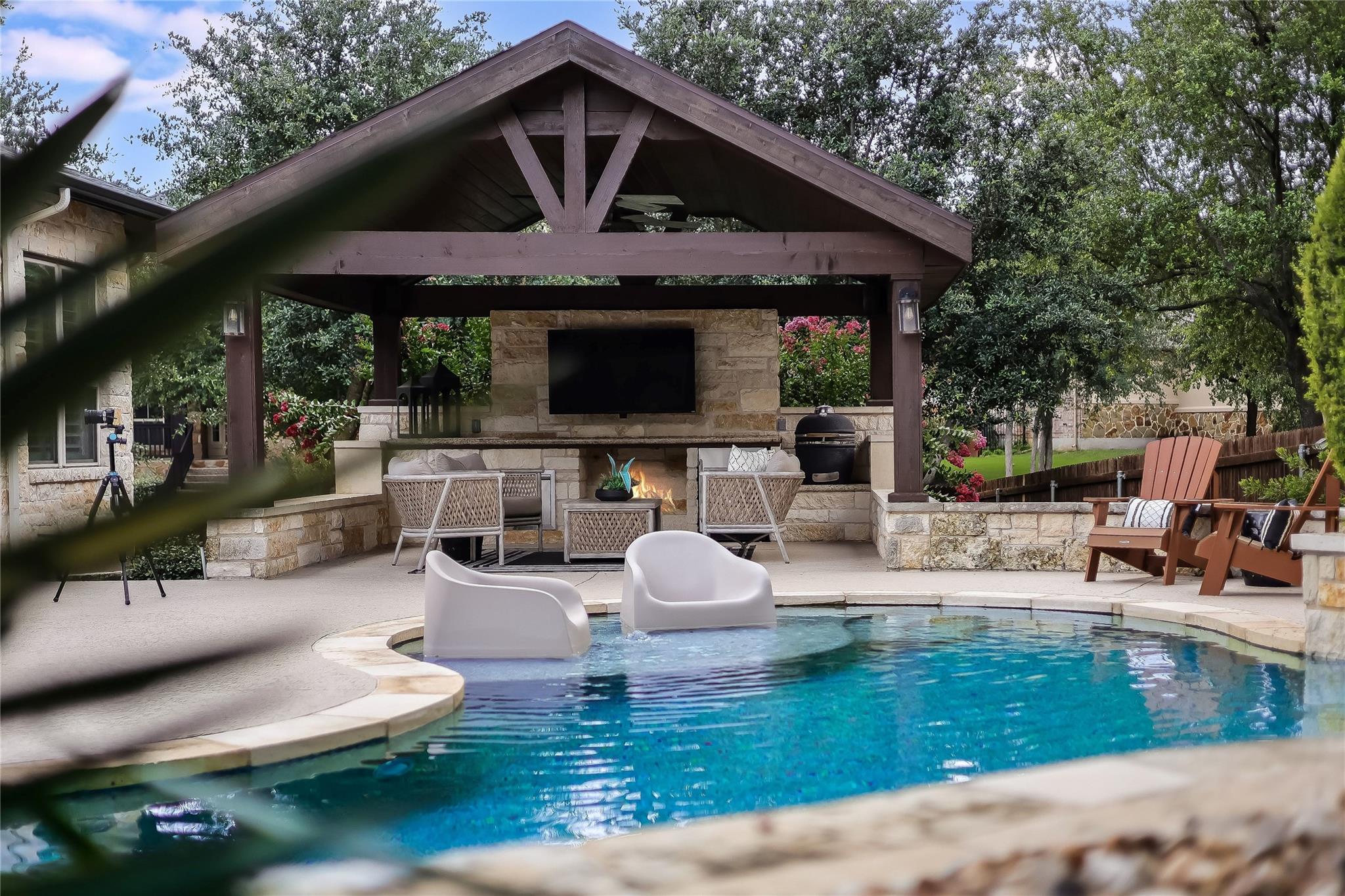
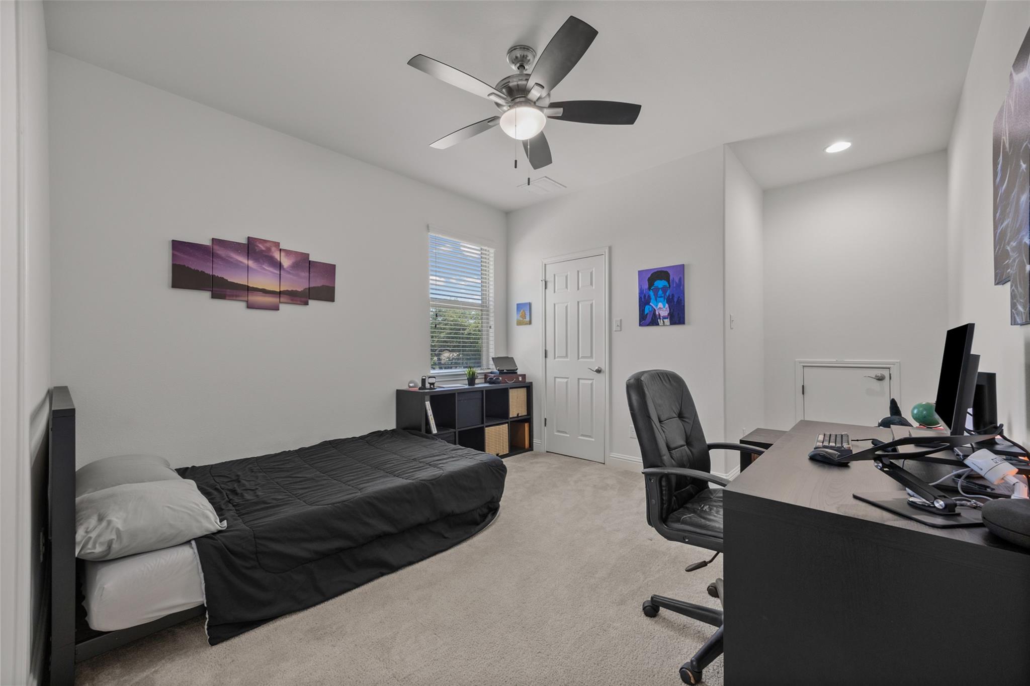
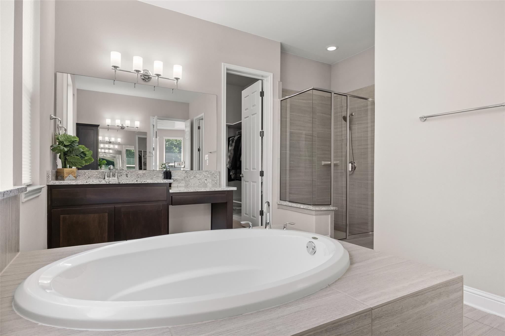
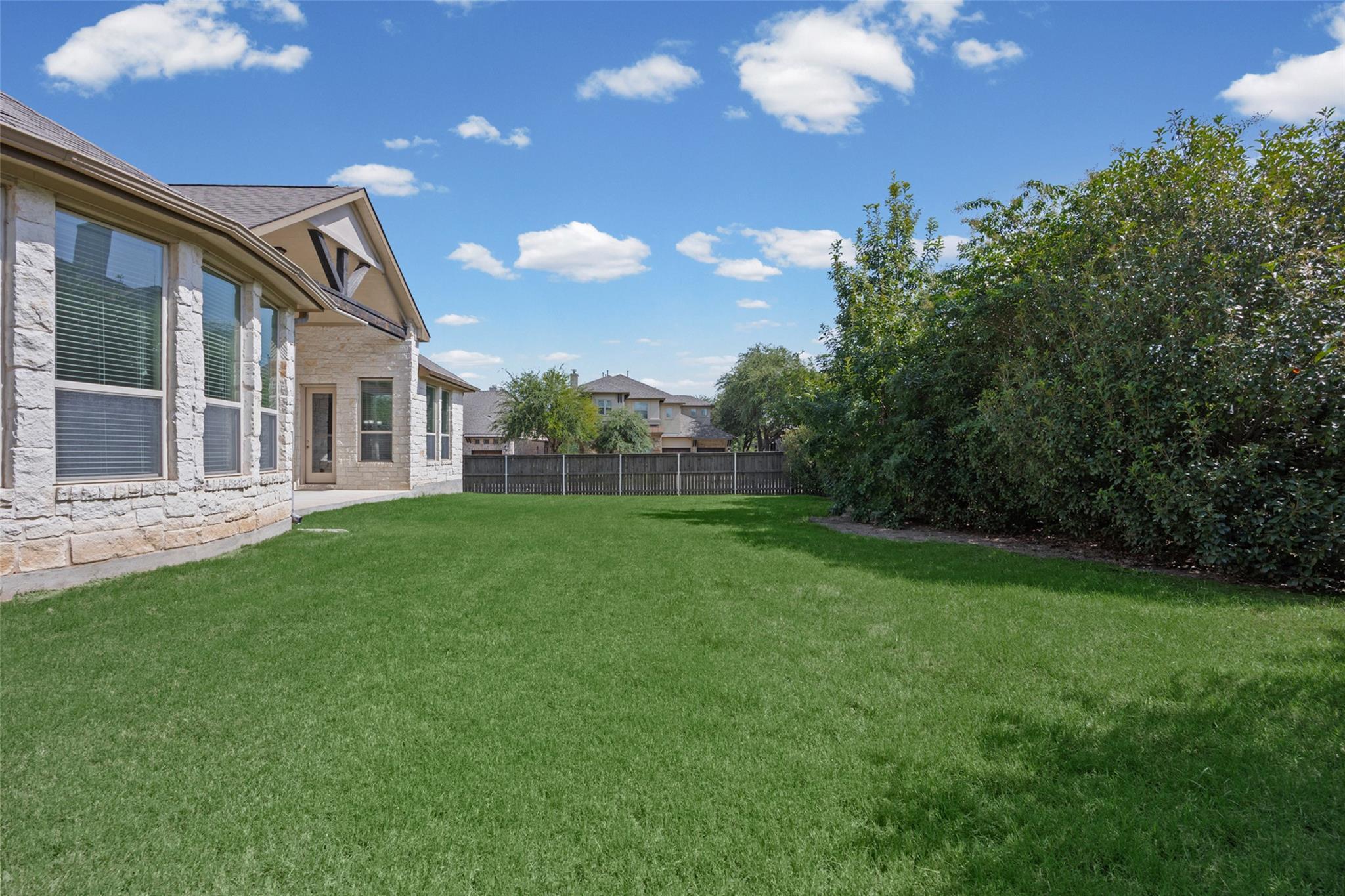
1 of the 1 photographs on this listing, chosen by ALEX Intelligence’s vision model — not from the MLS’s captions, which are generated. The 1 shown are the best examples of key property components that could be clearly identified.
Living area3,714 SFTwo stories
Bedrooms / baths4 / 3 + 1 half
Levels2
Garage3
Year built2010Typical for Ranch At Brushy Creek
Lot size0.21 ac9,108 SF
Days on market74Listed August 6, 2026; withdrawn October 19, 2026
Earliest new listingNovember 18, 2026Withdrawn October 19, 2026, plus 30 days.
Property details are from the ABOR MLS via secure APIs.
The land
Land values from Williamson Central Appraisal District
Land size can come from several sources: Williamson Central Appraisal District’s
tax records, the MLS listing, an appraisal or a survey. ALEX uses the one that best represents the land; where there is more
than one, the ALEX System defaults to the tax records (here the tax record carries
no lot area, so the MLS lot size is used). Land value defaults to Williamson Central Appraisal District.
If the land size sources disagree, discuss it with Diane.
Williamson Central Appraisal District values this parcel’s land at $187,000, but its record carries no lot area,
so no land rate per SF can be taken from it. Lot differences are priced from the adjustment schedule.
Click here for details
In plain terms. Each comparable is moved by the difference in lot size times one land rate
per SF, taken from the adjustment schedule, because the county has no land rate for this parcel.
How the land adjustment is computed
Model. Land is priced at a constant rate per SF of lot. For comparable
i the land line is
aᵢlot = (L − ℓᵢ) · λ, with
L this property’s MLS lot size (9,108 SF),
ℓᵢ the comparable’s MLS lot size, and
λ = land value ÷ (acres × 43,560) from this property’s own county
record.
The comparable’s own county rate is used only when this parcel has none; where neither exists the line is
zero and flagged (GEN-020) rather than estimated. No cap is applied. A line of 10% or more of the
comparable’s net sale price, |aᵢlot|/Pᵢ ≥ 0.10, raises a
variance notice (GEN-005) and changes no arithmetic. The table’s “Difference” is
ℓᵢ − L and “Share of net” is
|aᵢlot|/Pᵢ. The line is part of Aᵢ
and passes through the per-square-foot step like every other non-size adjustment.
Assumptions and limits
Assumptions. (i) Linearity. Every SF of lot is worth the same, the
5,000th and the 50,000th alike. The marginal value of land ordinarily falls as lots get larger, so an average
rate applied to a large difference tends to overstate it, and the bias is largest where the line is largest.
(ii) The county’s land value is a market value. It is a mass-appraisal figure set by schedule for
taxation; how closely it tracks what buyers pay for land is not tested here. (iii) One rate for the
set. This parcel’s rate is applied to every comparable, which suits a set drawn from one subdivision
and suits it less as the set spreads out.
What it cannot detect. Usable land is not lot area: slope, flood plain, easements, shape,
frontage and view are not in ℓᵢ and are not priced by this line, so two lots
of equal size can differ materially in value. The MLS lot size sets the difference and the county record sets the
rate. No interval is attached to λ: the
county publishes none, and none is invented.
Listing Pricing
Reduced once since listing
Listed August 6, 2026 at $1,245,000, reduced to $1,195,000 on August 24.
$900,000
$950,000
$1,000,000
$1,050,000
$1,100,000
$1,150,000
$1,200,000
$1,245,000
Original List PriceAug 6, 2026
−$50,000
$1,195,000
-4.0% from the originalLast Aug 24, 2026
−$275,100
$969,900
-22.1% from the originalALEX Recommended
List price
Reduction, $
Reduction, %
$ per SF
Original, August 6, 2026
$1,245,000
—
—
$335
Last, August 24, 2026
$1,195,000
−$50,000
−4.02%
$322
Total changes since original listing
−$50,000
−4.02%
−$13
Valuation
Both models start from the same sales. But at that point they
dramatically differ.
ALEX Model
Minimum$1,075,500
Average$1,065,936
Median$1,077,796
Maximum$1,230,520
Minimum held at $1,075,500.
That is 90% of the $1,195,000 last list price.
The lowest single sale indicates $978,325. Only the minimum moves; the average, median and valuation are the comparables’ own.
The ALEX Model uses five comparable sales. Each sale is
carried to this property’s 3,714 SF using the relationship between size and price
per SF that the model measures from 7,044
recent sales in the ABOR market: resales priced $1,000,000 and up, closed since July 2023.
The method is set out under “Click here for details” below.
Click here for details
In plain terms
Sales that are more like
this property — closer in size, age, lot size, room count and distance, and more
recent — count for more, and the way price per SF changes with size is
measured from the sales themselves rather than assumed.
What the method is called
Comparables are chosen by Mahalanobis-metric nearest-neighbor matching with
calipers (a caliper is a maximum allowed difference), and the valuation
is a kernel-weighted local linear regression — a local polynomial
fit, the same family as LOESS — evaluated at this property. Both run inside
ALEX’s valuation engine.
Which sales are admitted, and the boundary that is not drawn
The search starts as close to this property as the market allows. It tries the same
street within its subdivision, then the same phase or section, then the subdivision
family (every section and spelling of its name in this city, treated as one place). Only
when the tighter area holds too few usable sales does it widen, to rings of half a mile out
to five miles, and then to the ZIP code. It is not capped at
the subdivision. A hard boundary sounds safer than it is: where a subdivision has produced
four sales in two years, confining the model to them buys a tidy boundary at the cost of
a valuation resting on four houses. Where the pool does widen, every rule that widened
it is printed in this report, with how many sales each step admitted or dropped.
How far apart two houses are
Similarity is not distance on a map. Each sale is described by seven measurements:
living area in logs, year built, lot size in logs, distance from this property, months
since it closed, bedrooms and bathrooms. The Mahalanobis
distance combines all seven into one number, scaled by how much each varies in this
market and, where the market area holds enough sales to measure it, corrected for the
fact that they move together. Bigger houses tend to be newer and to sit on different
lots; a plain straight-line (Euclidean) distance would count what is largely one
difference several times over. Geography is one of the six, not the whole of it — a
near-identical house half a mile away is better evidence than a different house across
the street, and the metric says so.
The kernel, and why this one
Each admitted sale is weighted by an Epanechnikov kernel of its
distance: with u = d/h for bandwidth h,
the weight is 1 − u², reaching zero at the bandwidth
and staying there. (A bandwidth is the distance at which a sale stops counting.) Among non-negative kernels it is the one that minimizes
asymptotic mean squared error (Epanechnikov, 1969).
This is not the tricube kernel that LOESS uses by default, and not a
Gaussian one, and the difference matters at these sample sizes. In testing on six
comparables, tricube put 41% of the weight on one sale and 1.8% on another
— a six-comparable valuation actually resting on two. Epanechnikov falls away
gently enough that the set keeps contributing. The decay is quadratic and bounded, not
exponential: a sale past the bandwidth contributes nothing at all rather than a little,
which is what makes the admitted set an honest count.
The regression itself
With the weights fixed, the model runs a weighted least squares fit
of adjusted net price per SF on the logarithm of living area, and reads the
answer at this property’s size. Two things follow from that. The fit is
local: it is estimated for this property and discarded, and the next valuation
estimates its own. And the errors it minimizes are weighted, so the line is pulled
toward the sales that resemble this house and is allowed to miss the ones that do
not.
Two diagnostics are reported with every valuation. The bandwidth
says how far the model had to reach. The effective sample size says how
many comparables the weighting really amounts to: nine sales weighted 12% each is nine
pieces of evidence, while nine weighted 80/20 is closer to two. Where the effective
sample size is too small, or there are too few comparables, the model refuses to fit a
slope at all and falls back to a kernel-weighted mean of price per SF — the
Nadaraya-Watson estimator — rather than fitting a line the data cannot carry.
The size slope: measured on the wider market, read at these comparables
Price per SF is not flat across sizes: a larger house of the same kind
usually fetches less per SF. The model allows for this with a size slope, the change in
price per SF for each unit change in the logarithm of living area, and each comparable is carried to
this property’s size along it. A regression on the comparables alone has to estimate two things from
five or six sales: the level, this property’s price per SF at its own size, and the
slope. Five or six sales determine a level well and a slope badly. In ALEX’s backtest of
October 7, 2026, slopes fitted on the comparables alone had a median standard error of $74 per SF
per log-unit of living area against a median slope of −$125, so the uncertainty was more than half the
estimate; and where the house being valued was larger or smaller than every comparable, that poorly
determined slope was extrapolated beyond the evidence.
The slope is therefore estimated on a wider set of sales and held fixed, while the level is still read
from the comparables with their kernel weights. This is the mixed, or semiparametric, form of
geographically weighted regression: a coefficient that the local sample cannot pin down is
estimated over a wider area, and the coefficients the local sample can carry stay local (Fotheringham,
Brunsdon & Charlton, Geographically Weighted Regression, Wiley, 2002). The wider set is the
first of the following that holds at least 25 usable sales: this property’s subdivision family in its
city (every section and spelling of the subdivision’s name, together with the exact subdivision);
otherwise every sale within 2 miles; otherwise the whole market area searched for this valuation. A sale is
usable if it closed within the last 24 months, its living area is within 40% of this property’s, and
its year built and lot size are recorded. The slope is the partial ordinary-least-squares coefficient of net
price per SF on log living area, with year built, log lot size, bedrooms, bathrooms,
and months since sale held constant, so that it measures size rather than the newer construction or larger
lots that tend to come with it. Where no set qualifies, the slope is fitted on the comparables themselves, as
before; where even that is not supported (fewer than five comparables, or an effective sample size below
four), the fit is the kernel-weighted mean of price per SF.
On this property. The size slope is -96.4 dollars per
SF per log-unit of living area (standard error
59.7), estimated from 7,044 sales in
the ABOR market: resales priced $1,000,000 and up, closed since July 2023. A comparable 10% larger than this house therefore indicates about
$9 less per
SF before any other difference; fitted on the five comparables alone, the slope
would have been -7.3.
What it changed, measured. The test used 264 Williamson and Travis County single-family sales that
closed between April 7 and October 6, 2026. Each was valued as of its own closing date, from earlier sales only.
The market slope, together with the hold described next, lowered the median absolute percentage error from
7.06% to 6.10%. That is a paired difference of −0.96 points, 95% bootstrap interval −1.74 to −0.11
(ALEX backtest, October 7, 2026). The combination was chosen from about eighteen variants evaluated on the
same sales, so the improvement is probably somewhat overstated. The regression’s controls are not the
engine’s dollar adjustments, so an effect that moves with size, such as room count or lot, can be
counted in both places; the backtest measures the method with that overlap in it rather than assuming it
away.
Holding the valuation inside the evidence
Each comparable, adjusted for every difference but size and restated at this property’s size at its
own price per SF, indicates a value for this house. The ALEX Model then carries each
indication along the size slope and takes the kernel-weighted average. When this house is larger or smaller
than every comparable, the carry moves every indication in the same direction, and the weighted average can
land above the highest indication or below the lowest. A valuation there is one that no comparable supports
on its own. The committed valuation is therefore held inside the range of the indications:
if the weighted average lies outside it, the valuation is set to the nearer end, and this report states the
figure it replaced. The same rule is applied on the server, on this page whenever an agent edits a
comparable, and in the executive summary.
The rule has a measured cost. In the same backtest, the market slope without the hold placed 10.2% of
valuations outside their comparables’ indications and had the smaller errors in the tail: its mean
absolute percentage error was 1.44 points below the previous method (95% interval 0.64 to 2.34), against 1.09
points with the hold (0.38 to 1.87). The hold gives up part of that gain so that every valuation stays within
its evidence.
On this property. The hold does not apply under
the measured size effect: each sale is carried to this home’s size, so the weighted average of the carried
figures, $1,065,936, always lies between the lowest of them, $978,325, and the
highest, $1,230,520.
Transparent, and testable
Transparent because every step is written down in this report: which sales were
admitted, which were set aside and why, how each was weighted, and what was adjusted.
Testable because it is an estimator with stated assumptions whose accuracy is measured
by predicting each comparable from the others, and reported here whether or not that
flatters the figure. A number that can be checked is worth more than one that cannot.
Where the rest of it is
The full treatment — the exact kernel, the caliper widths, the effective sample
size, the bandwidth, the held-out test and the error band built from it — is set
out in The statistics.
Standard Arithmetic Model
Minimum$928,500401 Bluff Point Bnd
Average$1,007,050
Median$970,218
Maximum$1,161,389301 Raging River Rd
The same five sales, with no adjustments: each sale price divided by its SF,
averaged, times this property’s 3,714 SF, all from the MLS. Every sale counts equally.
How the two Models differ
Standard Arithmetic Model. The math is simple:
Sale Price per SF for Each Home Used as a Comparable Sale. For each home used as a comparable sale, divide its sale price by its total SF.
Average Sale Price per SF. Add the Sale Price per SF for Each Home, then divide by the number of homes.
Your Home’s SF. Use the SF on the MLS listing, the same source as every comparable sale.
Your Home’s Estimated Value. Average Sale Price per SF multiplied by Your Home’s SF.
Example. $200 (Average Sale Price per SF) × 2,500 SF (Your Home’s SF) =
$500,000 (Your Home’s Estimated Value).
ALEX Model. It is statistically sound and accurate:
Comparable Sales. Closed sales like Your Home, chosen by ALEX’s selection rules or by the agent.
Net Sale Price for Each Home Used as a Comparable Sale. Its sale price less the closing costs and repairs the seller paid, as recorded in the MLS.
Time Adjustment. Each net sale price is brought to today with ALEX’s repeat-sales index for the county.
Feature Adjustments. Each difference from Your Home — bathrooms, garage, lot size, view, age and the rest — is priced at what ABOR closed sales in the same price range show the market pays.
Price per SF. Each adjusted price is divided by the sale’s own SF.
At Your Home’s Size. That price per SF is multiplied by Your Home’s SF, then corrected because larger homes sell for less per SF, as measured on the market.
Weighting. Sales most like Your Home count for more, whether ALEX or the agent selected them. Each sale’s weight is shown in the report.
Your Home’s Estimated Value. The weighted average of the sales (a plain average when they count equally), with the minimum, median and maximum beside it.
How one sale becomes a value: 204 Broken Arrow Dr
Sale price
$1,015,000
What it sold for
Net sale price
$1,013,000
−$2,000
Less the buyer's closing costs and repairs the seller paid
Brought to today
$980,645
−$32,355
The market's change since it sold
Adjusted to this home
$1,018,705
+$38,060
ALEX's measured adjustments for every difference
Price per SF
$251.53/SF
Its adjusted price divided by its own 4,050 SF
At this home's size
$934,190
−$84,515
Its adjusted price per SF times this home's 3,714 SF
Size correction
$978,325
+$44,135
Larger homes sell for less per SF, measured on the market
This sale
says this home is worth $978,325 and carries 27.9%
of the weight, the most of the five sales, because it is the closest match. Every sale goes through the same steps.
The weighted average of all five is $1,065,936. That is ALEX’s valuation.
How much each sale counts
204 Broken Arrow Dr
$978,325
27.9%
305 Stiles Cv
$1,079,046
26.7%
401 Bluff View Rd
$1,045,142
17.4%
401 Bluff Point Bnd
$1,077,796
14.2%
301 Raging River Rd
$1,230,520
13.9%
Weighted average
$1,065,936
100%
Each slice is one sale’s share of the valuation. The closer a
sale is to this home on the seven measures of similarity, the bigger its slice. The dollar figure is what that sale says
this home is worth. Each one is multiplied by its share, and the results add up to the weighted average.
ALEX Model valuation is $58,886
higher than the Standard Arithmetic Model —
5.8% higher.
ALEX Model$1,065,936
Standard Arithmetic Model$1,007,050
The ALEX Model is$58,886higher
The ALEX Model is5.8%higher
The statistics
Overall Error Score (RMSLE)0.0847One score for all 5 test runs together, counted in proportions rather than dollars.
Forecast Standard Deviation9.5%How widely the held-out predictions scattered around the actual net sale prices, in proportional terms.
68% Error Band±8.1%Calibrated on 145 past Williamson County sales valued the same way: 68% came this close to the actual net sale price.
Median Error (MdAPE)3.8%The middle miss. Half the test runs were closer than this, and half were farther.
Within 10% (PPE10)60%How often a test run came within 10% of the actual net sale price.
Held-out Tests5Every figure on this row is measured on this many comparable sales.
Click here for details
Forecast standard deviation (FSD) — defined
In plain terms
How widely predictions
made by this method scatter around actual sale prices. Lower is better. If the errors are
roughly bell-shaped, an FSD of 9.5% means about two in three
predictions land within 9.5% of the actual price and one in three
further out. It is measured on this property’s own comparables, so it describes the
spread of the evidence here — not a promise about the price this house will fetch.
Formula. Each comparable in turn is hidden and its net sale price
Pᵢ is predicted from the others as P̂ᵢ.
FSD is the sample standard deviation of the log ratios:
FSD = √( Σ (dᵢ − d̄)² / (n − 1) ), with
dᵢ = ln(P̂ᵢ / Pᵢ). Here
n = 5 and FSD = 0.0945.
How to read it. Lower is better. FSD is the measure automated valuation model (AVM)
providers commonly publish with their estimates, so it can be compared with theirs in definition — with
the caution that theirs is measured on thousands of sales and this one on 5.
Overall error score (RMSLE) — defined
In plain terms. One number that sums up how far off the predictions were across all the
held-out comparables, treating a miss of a given proportion the same whether it was high or low. Lower is better; 0 would be
perfect. This property scores 0.0847.
Formula. Root mean squared logarithmic error,
RMSLE = √( (1/n) Σ (ln(1 + P̂ᵢ) − ln(1 + Pᵢ))² ),
over the same 5 held-out predictions. Because it works on logarithms, it
measures proportional error, and because it squares each miss, one large miss raises it more than several
small ones.
How to read it. RMSLE has no upper bound and no threshold: it starts at 0, which
would be perfect prediction, and rises without limit, so lower is always better. Because it is measured in
logarithms, its value reads roughly as a proportion — 0.10 corresponds to predictions typically about
10% off, and 1.0 would mean being wrong by a factor of about 2.7. This property scores
0.0847. It is most useful for comparing one method against another on the same sales,
rather than read on its own.
Median error (MdAPE) — defined
In plain terms
Line the held-out misses up
smallest to largest and take the middle one. Half were closer than this, half further. It is
the typical miss, and unlike an average it does not move when one comparable is badly
wrong.
Formula.MdAPE = medianᵢ |P̂ᵢ − Pᵢ| / Pᵢ,
over the same n = 5 held-out predictions, expressed as a percentage:
3.75%. The mean of the same errors (MAPE) is
6.73% and the largest single one is
12.91%.
Why it is here, beside RMSLE. The two answer different questions and are
reported together deliberately. RMSLE squares each miss, so it is carried by the worst
comparable; MdAPE is a median, so it is carried by none of them. A set with four close
comparables and one poor one shows a low MdAPE and a raised RMSLE, and that gap is itself the
finding — it says the method works on this property except on one sale, which is worth
knowing before the gap is averaged away. Where the two agree, the error is spread evenly
through the set.
What it does not say. With n = 5, the median is
one of 5 numbers, not an estimate of a population median: change one comparable and it can
move to the next order statistic. It is the typical miss on this set, not the typical
miss of the method.
Within 5% and within 10% (PPE5, PPE10) — defined
In plain terms
How often the method landed
close. Of the 5 hidden sales, 3 came within 5% of what the house actually
sold for and 3 came within 10%. The range after each one says how far those
shares could reasonably be off, given how few sales they are measured on.
Formula.PPEk = (1/n) Σᵢ 1[ |P̂ᵢ − Pᵢ| / Pᵢ ≤ k ]
— the share of held-out predictions inside a tolerance of k. Here
PPE5 = 3/5 = 60% and
PPE10 = 3/5 = 60%. These are the
industry’s own yardstick: PPE10 is what vendors quote as “within 10%”.
The interval, and why it is not optional. A share measured on 5 trials can
only take the values 0%, 20%, 40%, 60%, 80%, 100% —
it moves in steps of 20 points, so the figure alone would claim a precision the
sample cannot carry. Each is therefore reported with a Wilson score interval at 95%:
( p̂ + z²/2n ± z√( p̂(1−p̂)/n + z²/4n² ) ) / (1 + z²/n)
with z = 1.96. Wilson rather than the textbook
p̂ ± z√(p̂(1−p̂)/n) because that interval
collapses to zero width at p̂ = 0 or 1 —
a run of 5 hits would report certainty — and its coverage is poor at small
n (Brown, Cai & DasGupta, 2001). Wilson stays inside
[0, 1] and keeps its nominal coverage here.
PPE5 is 23% to 88%,
PPE10 23% to 88%.
The width of those ranges, not the shares inside them, is the honest summary of what
5 held-out sales can establish.
What is not claimed. The tolerances are fixed at 5% and 10% before the errors are
seen, never chosen to flatter the result. And a share is a blunt instrument by construction: a miss of
5.1% and a miss of 50% both count as outside, which is why MdAPE and the error band are reported beside
these and not instead of them.
Cross validation — the error measured on this property
Which figure these
measures belong to. Every error and band here is computed for
ALEX’s valuation of $1,065,936 —
the same net sale price shown at the head of the report, on the same basis: what the seller
keeps after paying the buyer’s closing costs and any repair credit. It is not the
grossed-up contract price quoted against the outside estimates in Benchmarks. If an agent has
changed an adjustment, the figure at the head of the report moves; these measures do not move
with it, because they measure how ALEX’s method performed on this property, not how a
revised figure would perform. A changed valuation carries no measured band until the change is
tested the same way.
How this was tested, in one sentence: each of the
five sales was set aside in turn, its net sale price was predicted by this same method from
the other four alone, and the prediction was compared with what
that sale actually netted — five tests, one for each sale. This is called
leave-one-out cross-validation.
Five tests is a small number from which a spread can be quoted.
These figures are real and specific to this house, but thin: one unusual comparable moves them
materially. Treat them as the shape of the uncertainty, not a precise measurement of it.
68% error band0.0808calibrated on 145 salesThis method was run on 145 past Williamson County sales, each valued as of its
own closing date from earlier sales only, and 68% of those values came within
±8.08% of the actual net sale price. Applied to this
valuation that is ±$86,128, or $979,808 to
$1,152,064. The 95% band is 0.1970:
±$209,989, or $855,947 to $1,275,925. This property’s own
five tests put the 68th-percentile miss at ±10.17%; that is too
few tests to set a band, so it is shown as a check only.
Typical spread — FSD9.45%±$100,773 on this valueHow widely the held-out predictions scattered around the actual net sale prices. It is the same
measure Zillow (5%) and HouseCanary (5%) publish for their own models on this property,
computed on very different samples.
RMSLE0.0847lower is betterA single overall error score in proportional terms, so an expensive sale does not
count more than a modest one. Because each miss is squared, one large miss raises it more than
several small ones. It is mainly for comparing one method against another.
Median error3.75%mean 6.73%, worst 12.91%The middle of the misses — the most direct answer to
“how far off is this method typically”.
What happened when each sale was hidden and predicted from the others: how far off that prediction was, as a share of what the sale actually netted. Past 10% is red.
Held out
Actual net
Predicted from the others
Error
204 Broken Arrow Dr
$1,013,000
$1,141,309
+12.67%
305 Stiles Cv
$996,999
$965,008
−3.21%
401 Bluff View Rd
$1,069,000
$1,057,296
−1.09%
401 Bluff Point Bnd
$1,132,000
$1,174,484
+3.75%
301 Raging River Rd
$1,425,000
$1,240,980
−12.91%
Converting a net price to a contract price
In plain terms
The valuation is a net figure: what a seller keeps after the credits a buyer customarily asks for. A contract is written at a higher number that nets down to it. This explains the conversion between the two, so neither is mistaken for the other.
Why there are two, and where each is used. This valuation is a net sale
price. Two places in the report need a contract price instead, and they do not use the same
conversion, so both are stated here rather than left to be discovered.
One: the neighborhood ratio, used for comparison.ρ̂ = median(net / close) over closed sales in
Ranch At Brushy Creek (the subject's subdivision)
in the last 24 months, n = 75, with a minimum of 15 sales before the level is used at
all. Here ρ̂ = 0.9987, an implied
seller contribution of 0.13% of the contract price. It
grosses our net figure up for the Benchmarks comparison and sets the “how far above the
evidence the asking price sits” percentage. It is a median of ratios, unweighted, with
no interval reported: at n = 75 a median carries real sampling error, and none is
claimed for it.
Two: the pool share, used for the offer ladder.ŝ = Σwᵢ(Cᵢ+Rᵢ)/Pᵢ ÷ Σwᵢ,
a recency-weighted MEAN of the actual contribution share over the negotiation pool, with its
own drawer in the recommendation section. The two differ in three ways:
Estimator: a median of a ratio, against a weighted mean of a share.
Pool: a subdivision, or its city, over 24 months, against resales in this property’s ZIP code
asking within 15% of its price.
What they measure: net divided by close, which includes anything that separated the two, against
closing costs and repairs specifically.
What that means for a reader. The two conversions do not have to agree; on this property the pool share could not be computed, so no
difference between them is stated. Neither is used to alter the valuation itself, which
is and remains a net sale price. Where a contract price appears, the conversion behind it is
named in that section.
The page’s closing-cost control uses a third. Where this page converts the valuation
to a contract price from its closing-cost control, it uses
C = (V̂ + R)/(1 − c), rounded to $500, with c the
closing-cost share and R the repair credit set in that control, which starts from the
negotiation pool and which the agent can change. It is not
ρ̂. Grossing by
ρ̂ for the Benchmarks comparison gives
G = V̂/ρ̂ = $1,065,936 ÷ 0.9987 = $1,067,324.
Assumptions and limits of ρ̂. The sample is every closed
sale with a positive close and net price whose subdivision name begins with
Ranch At Brushy Creek, with no filter on property
type, condition, price band or arm’s-length status beyond what the warehouse table already applies; a
neighboring subdivision whose name shares the prefix is included. A median of ratios is not the ratio of
medians and ignores how large the contributions were: where most sales carry none,
ρ̂ can be exactly 1 while a minority carried large ones. A sale whose concession
was never recorded in the MLS fields enters at a ratio of 1.
How the comparables were chosen
Why this matters for everything above. The held-out error, the bands and
the confidence score all rest on the comparables actually chosen. If the selection rule were
unstated, a reader could not judge whether the held-out comparables and the subject are alike
enough for the error measured on them to say anything about the subject. The rule is
therefore stated in full, in the order it runs.
The method, named. Selection is Mahalanobis-metric nearest-neighbor
matching with calipers (Rubin 1980, Biometrics 36:293; Rosenbaum & Rubin 1985,
The American Statistician 39:33; Abadie & Imbens 2006, Econometrica
74:235), run inside an ordered set of geographic strata. The strata decide where
this market is; the metric decides which sales inside it are comparable. This
replaced an earlier cascade of fixed search criteria that stopped at the first rung holding
six candidates and then ranked them on a weighted score of stated conventions. Two
differences matter: the cascade treated any two sales clearing the same rung as equally
comparable, and when a rung ran short it widened the living-area band to as much as
±45% — producing candidates this valuation’s own ±25% standard then
discarded. Selection now cannot hand the estimator a sale the estimator must refuse.
Step 1 — what is removed before anything else. Sales that are not
arm’s length (bank-owned (REO), short sale, auction, HUD, corporate-owned and probate
sales, identified from the MLS listing conditions and the listing remarks), sales in fair or
poor condition, sales in a FEMA flood zone, sales whose net sale price is more than
±20% from this property’s asking price (where it has one), and this
property’s own earlier sale. That earlier sale can be readmitted only when fewer than
three other comparables are available, and then only if it was arm’s length, closed at
least 12 months ago and can be carried to today on the price index.
Step 2 — admissibility. These are the differences a distance must
never be allowed to trade away. Each is categorical: a two-story house is not a one-story
house that happens to be far away, and no dollar adjustment converts one into the other. Each
rule below is applied in order, to what the rule above it left.
The first four are hard: they are
never relaxed, even when relaxing them is the only way to field a comparable, because a
valuation with no comparable is a problem an agent can see and a valuation built on the wrong
product is one nobody sees.
The rest are relaxed only if applying them would leave nothing at all, and any such relaxation
is named in the table.
Rule
What it requires
Why it is a rule and not an adjustment
Sales in
Excluded
Left
Age-restricted community hard
A sale in an age-restricted (55+) community may be compared only with another such sale, and never with one outside it. Read from the MLS restrictions field where the feed supplies it, and from a curated list of named communities where it does not.
A 55+ community is a different product with a different buyer pool, and no dollar adjustment can undo it. The rule exists because of an earlier Georgetown valuation: the search reached five miles, took five Sun City comparables carrying a $1,960 annual HOA that property did not have, and came back $42,000 low. The MLS senior-community flag is filled in on none of 535,397 listings, so the feed alone cannot catch this.
25
—
25
Association fee hard
Annual association dues must be within the stated gap of this property's.
Dues are a recurring cost capitalized into price. The gap also catches amenity-heavy communities the age rule has not named.
25
—
25
School district hard
Same school district. A comparable with no district recorded is admitted.
District boundaries are a documented price discontinuity and they do not follow distance: two houses a street apart can sit in different districts.
25
−3
22
Elementary school hard
Same elementary school as this property, as the MLS listing names it. A comparable with none recorded is admitted.
The elementary attendance zone is the finest school boundary in the feed and moves price as much as the district does; it can split one subdivision (George, 2026-10-17: hyper critical).
22
—
22
View
Same view category as this property.
A greenbelt view and a lake view are separate markets, not a difference in degree.
22
relaxed
22
Attached or detached
Attached homes compare only with attached, detached only with detached.
Shared walls change the buyer pool, the insurance and the land interest. It is a different product, not a nearby one.
22
—
22
Stories
Single-story compares with single-story, multi-story with multi-story.
Single-level living commands its own premium in this market and is the first filter many buyers apply. The engine adjusts for story type within a match; it cannot convert one into the other.
22
−1
21
Waterfront
Waterfront compares only with waterfront.
Water frontage is a land interest, not a feature, and its premium varies by body of water rather than by a rate that could be applied.
21
—
21
New construction
New construction compares only with new construction.
A builder's first sale carries incentives, warranty and finish that a resale does not, and it is priced off a price sheet rather than off the market.
21
—
21
Pool
If this property has no pool, comparables with a pool are excluded. If it has one, both are admitted and the difference is adjusted.
The rule is deliberately one-sided. The engine does adjust for a pool, but when the subject has none, every indication would then rest on that one adjustment.
21
—
21
Builder
For a new-construction subject with a named builder, comparables naming a different builder are excluded. A comparable with no builder recorded is admitted.
Builder premium runs 8-12% within one subdivision. Missing data is treated as admissible rather than disqualifying, because the MLS fills this field sparsely.
21
—
21
Sale-to-list
Net sale price between 0.93 and 1.03 of the comparable's own list price.
A sale far off its own asking price is usually a data error, a related-party transfer or a term the concession fields do not record. Note this tests the sale against ITS OWN list price, never against this property's price.
21
−1
20
Lot density
Living area per acre within a factor of 3.0 of this property's.
It separates product types that size and lot size do not: a 2,000 SF house on a quarter acre and the same house on five acres are different markets.
20
—
20
Relaxed for this property: View. Applying
it would have left no comparable at all, which means
that rule has stopped describing this
market rather than that the difference stopped mattering. Read the valuation accordingly.
Step 3 — the market area, tightest first. The remaining sales are
placed in nested strata. First the same street in this subdivision, then the same phase or section,
then the subdivision. The subdivision is taken as every subdivision sharing its name in this city.
So a “Serenada West” sits with “Serenada” and “Serenada
Estates”: the distinction between them is a platting artifact, not a market boundary.
After the subdivision come half a mile, one, two, three and five miles, then the postal code. The shared name
must be distinctive on its own: a first word under five letters keeps its second, so
“Sun City” never collapses to “Sun” and sweeps in Sunrise.
The search stops at the tightest stratum holding at least five eligible sales
— eligible, not merely present, and five because that is the number the estimator
is built on. A subdivision holding five admissible sales is not abandoned for a
one-mile ring holding six: that trades the definition of the market for one more
observation, which is the wrong trade. Counting eligible sales rather than candidates
also corrects an old fault: the earlier rule stopped at the first rung holding six candidates, and the valuation then discarded those outside its size
standard and finished on three. The rung looked full and the report was thin.
Step 4 — the hard calipers. A sale is eligible only if its living
area is within ±25% of this
property’s — the same appraisal size standard the valuation itself applies, so the
two can never disagree — and only if it closed within the time window. The window opens
at 13 months, which guarantees a full seasonal cycle, and widens to 24 only when 13 cannot
fill the stratum. Time widens before geography: a sale two streets away eighteen
months ago is better evidence than a sale two miles away last month, because the repeat-sales
index can carry a date and nothing can carry a different market.
Inside this property’s own subdivision — the same street, the same phase and the subdivision as a whole —
the window can reach further, back to August 1, 2022, but only after every one of those rungs has failed to fill at 13
and at 24 months. Comparable sales come only from this subdivision; a wider area is searched only when the
subdivision holds no eligible sale since August 1, 2022, and the report says so. July 2022 is when this market changed: as mortgage rates rose from 3.1% to 5.5%, July 2022 was the
first month ABOR single-family homes no longer sold above their original list price (100.0%, from 104.5% in April)
and the median time on market doubled, so sales after it belong to the market that exists today and earlier ones do
not. Tested on 142 Williamson and Travis County sales from April to October 2026, each valued only from sales
before it, the rule changed the comparables of 13, all of which then came entirely from their own subdivision, and
lowered the median absolute error from 5.57% to 5.27% (sales valued within 5% of the price: 43.7% to 47.2%).
This
report used a 13-month window.
Step 5 — the distance itself. Each eligible sale is placed in a
7-dimensional space
— living area (logarithm), year built, lot size (logarithm), distance from this property, in miles, months between the sale and today, bedrooms, and bathrooms —
and its distance from this property is measured as
d² = (xᵢ − x₀)′ Σ⁻¹ (xᵢ − x₀),
where Σ is the covariance of those covariates across every
admissible sale in the market area. Estimating Σ on the market
rather than on the handful of sales in hand is what makes the distance mean something: two
hundred SF is a large difference in a tract of identical houses and nothing in a
custom one. Each variance is inflated slightly (5%) before inversion, a simple form of the shrinkage
idea in Ledoit & Wolf (2004), so the inversion stays stable; where the market area holds
fewer than five sales per covariate the off-diagonal terms are dropped and the measure becomes
standardized Euclidean distance, which is the same statistic when the covariates are
uncorrelated. The basis line records which was used.
Mahalanobis distance on 7 covariates (metric from 49 sales in the market area), within Ranch at Brushy Creek, all phases and sections; 6 of the 16 sales there clear the size and time standards, 5 of those are inside the distance caliper, 13 months of sales considered
The caliper, and the factor of two in it. A sale is admitted when
d² ≤ 2χ²p,0.5, the median contour of the
reference distribution. The factor of two is not a tuning choice: the subject is one draw and
the comparable another, so their difference has covariance
2Σ and d² is distributed as
2χ²p, not χ²p.
Calipering at the plain χ² median — the error this
model carried until it was measured — admits only the nearest sixth of an honest pool.
For this report the caliper is
d² ≤ 12.69.
The caliper excludes only while exclusion still leaves five comparables. Below that the
nearest sales fill the set and each one past the caliper is named, because a sixth constraint
that silently cuts a valuation to three is not a better valuation.
This property, in numbers. 49 closed sales survived
step 1, 20 of them admissible under step
2, 6 eligible inside the chosen
stratum after the size and time calipers,
5 inside the distance caliper, and
n = 5 used.
What is deliberately NOT a selection rule. The old cascade filtered on
price per SF and gave it weight in its ranking score. That is the very quantity the valuation goes on to average, so choosing comparables for
already agreeing on it narrows the measured dispersion by assuming the answer. It has been
removed. Nothing in selection now looks at the comparable’s price except the
±20% asking-price screen in step 1 and the sale-to-list test in step 2, and that test
compares each sale with its own list price, never with this property’s.
Outliers are handled after adjustment, where they can be seen and named.
After selection, two further rules. (1) Same neighborhood.
When at least three of the selected comparables share this property’s subdivision
family, only those are kept.
Family, not the recorded plat name: matching on the exact name made this rule fight the
selection ladder above it, throwing out the sibling sections that ladder had just brought
in. (2) Size. The set used is
K = {i : |sᵢ/S − 1| ≤ 0.25}; if that holds fewer than five, the band is
widened to ±30% and then ±35% only as far as needed, and if fewer than three remain even
then, every comparable with a known living area and net price is used; here none was set aside.
The final set is n = 5.
Where the agent stands in this.
The comparables on this
page are the model’s own. An agent may replace or remove any of them, and the report
then records that it was an agent’s set. A comparable an agent adds by hand carries no
computed distance and is given full weight in the estimator, deliberately: the agent has
asserted it is comparable, and that assertion is the best evidence available about it.
The limit this creates, stated plainly. Selection is not random. The five
sales are the closest matches the rule could find, which is what makes them useful evidence
and also what makes the leave-one-out error an optimistic estimate of the error on an
arbitrary house: a held-out comparable is being predicted by four sales chosen to be like it.
Removing the price-per-SF filter narrows this bias but does not end it: sales alike in size,
age, lot and location are alike in price, so selection still favors agreement.
The population figures in this section, measured on a blind holdout of sales the model never
saw, are the more conservative answer to the same question. Both are printed for that reason.
The evidence-quality score
In plain terms
A score out of 100 for how good the evidence behind the valuation is: how many comparable sales there were, how similar, how recent, and how much they had to be adjusted. It rates the evidence, not the house.
What it scores. 67 of 100 scores the EVIDENCE behind
this valuation, not the property and not the probability that the figure is right. It is an
index built from four factors, each worth up to 25 points with a floor of 12, because even a
weak signal carries some information:
Factor 1, how tight the market area had to be. The model walks a ladder
of geographic strata from tightest to widest — the same street, then the phase, the
subdivision, then half a mile out to five, then the postal code — and stops at the
tightest one holding enough eligible sales. The score is that stop’s position on the
ladder, linearly: the tightest rung earns 25, the widest 12. The stratum used is named in the selection drawer.
Factor 2, the back-test error. One point deducted per percentage point of
leave-one-out error, flooring at 12 once the error reaches 13%. The factor is a restatement of
measured performance, not a second opinion about it — measured by the valuation engine on
its own proposed set, which is not necessarily the table above (see the cautions below).
Factor 3, how recent the comparables are. One point deducted per 15 days
of average age across the set, flooring at 12 once the average passes 195 days.
Factor 4, how much adjustment was needed. One point deducted per
percentage point of average absolute adjustment as a share of each comparable’s net
price, flooring at 12 at 13%. A set that needed little adjustment scores higher than one
rebuilt line by line.
When a factor cannot be measured. It is omitted rather than filled in, and
the remaining factors are averaged and scaled to the same 100-point frame; the valuation
records which factors were measured. A score built from two real factors is reported as such
rather than padded to four with invented inputs.
The tightness bonus and the cap. A set drawn from the top of the ladder
earns up to 15 additional points — 15 on the same street, 10 in the same phase, 5 in
the subdivision, nothing beyond it — and the total is then capped at 100. The bonus
covers exactly the rungs that are the same market rather than merely nearby. Labels: high at 70 or above, medium at 50 or above, low below 50 —
this property scores 67, medium.
Formally. With τ the stopping stratum’s position on a ladder
of T strata (0 the tightest), ē the engine’s mean
held-out error in percent, ā the mean comparable age in days and
ḡ = n⁻¹ Σ 100|Σₖ aᵢₖ|/Pᵢ:
f₁ = round(25 − 13τ/(T−1));
f₂ = max(12, 25 − round(ē));
f₃ = max(12, 25 − ⌊ā/15⌋);
f₄ = max(12, 25 − round(ḡ)). Over the m factors
that could be measured, Q = min(100, round(4Σf/m) + B), with
B = round(15(1 − τ/3)) for τ < 3
(the same street, the same phase, the subdivision) and 0 otherwise.
Two cautions the formula makes visible. Factor 4 takes the absolute value of the
net adjustment, |Σₖ aᵢₖ|, so offsetting lines cancel and a
heavily adjusted comparable can score as lightly adjusted — the opposite choice from the gross measure in
the provenance section, and the weaker one. And the score is computed by the valuation engine on its own proposed
set and its own held-out test, before this report applies the same-subdivision rule, the ±25% size standard
and the per-square-foot average: ē therefore need not equal the median error in the
table above, and the score is not recomputed when the agent edits the set.
What it is not. The deductions above are conventions chosen so the score
moves in the right direction and can be read off the inputs; they are not fitted coefficients,
the score has no sampling distribution, and no interval is attached to it. It is not a
probability and must not be read as one. The uncertainty this report measures is the
held-out error and the bands built from it, above.
How the population figures were produced. They come from the training
run’s own artifact, not from this page: a single temporal split, train on everything
closing on or before 2026-03-30 and test on the
6 months after it, so no sale in
the test set was seen in any form during fitting. The test set holds 19,621
sales out of the full table.
Leases are removed, and the metrics are reported segmented by property type and price band as
well as overall, because a single blended figure hides exactly the segments that matter.
No interval is attached to these population figures in the artifact, and none is invented
here.
What they do and do not describe. They describe the ALEX statistical
model across a metro-wide holdout. They are not the accuracy of the comparable-sales figure
on this page, which is measured by leaving each comparable out, immediately above; the two
are different estimators on different samples and are reported separately for that reason.
Part one — what a valuation should be measured against
This section is reserved. The standard is
being supplied separately and will be placed here in full. It is deliberately empty
rather than filled with a plausible-looking threshold: a benchmark that this report happened
to pass would be indistinguishable, to a reader, from one it had actually been measured
against. Until the paper is here, no accuracy standard is being claimed or implied anywhere
in this report.
What is known today, pending that standard. Three sets of numbers exist
and none of them is a standard — they are measurements, and they are not measuring the
same thing:
1. This property. Median error 3.75%, FSD
9.45%, RMSLE 0.0847, 68th-percentile miss
±10.17%, from five held-out comparables. Specific to this house, and
thin: five observations describe this comparable set accurately and generalize weakly.
2. This model, across its blind holdout. MdAPE 8.19%,
MAPE 11.45%, RMSLE 0.1652 over
19,621 sales the model never saw during training. This is the right basis for any general claim about the
method, and it is deliberately not what the tiles above report — those answer “how
accurate is this valuation”, which is a different question.
3. What the vendors publish for themselves. As self-reported by each vendor
(figures they revise from time to time, not independently verified here): HouseCanary, national MdAPE
2.8% over 1,994,203 transactions internally and 2.9% on a blind
third-party test; Zillow, median error 1.79% for homes on the market and
7.20% off the market. Two cautions before either is treated as a bar to clear.
Both are national aggregates dominated by dense, homogeneous tract housing where an automated
model does best, and neither is conditioned on the kind of property this is. And the
on-market figure is not independent of the asking price — both vendors use the list
price as an input, which is the point made in the Benchmarks section.
What a standard would need to specify to be usable here. The forthcoming
paper will presumably settle five questions:
which statistic is the criterion (MdAPE, FSD, coverage, or a hit rate);
whether it is a point threshold or a distribution;
whether it applies per property or per portfolio;
how it is conditioned on price band, property type and evidence depth;
whether an interval must be calibrated: whether a stated 68% interval must actually
contain the outcome 68% of the time.
The last is materially stricter than a median error threshold. It is also the one most AVM
disclosures avoid.
Where this report already goes beyond common practice, whatever the standard
turns out to be: the comparables are named, every adjustment is itemized with its reason,
the estimator and its weights are stated, and the held-out test results are printed so
every summary statistic can be recomputed by hand. A standard can be applied to a number; it
can only be verified against a number whose derivation is visible.
Part two — how this valuation was measured
Why hold anything out at all. Scoring a method on the same sales it was
given measures how well it can interpolate data it has already seen, which is not the
quantity anyone cares about. The quantity of interest is expected loss on an observation
drawn from the same population and not used in fitting:
Err = E(X,Y)[L(Y, f̂(X))]. Resubstitution error is
downward-biased for it by construction.
Design: leave-one-out cross-validation. The adjustments
Aᵢ are ALEX’s per-comparable adjustments to this property
(repeat-sales time carry included, the plain living-area line excluded), giving each comparable an
adjusted value per SF rᵢ = (Pᵢ + Aᵢ) / sᵢ. For
i = 1,…,n comparable i is removed and the
weighted fit is re-run on the rest, re-centered on i so the kernel weights are
distances from i rather than from this property. Writing
r̂−i for that fit read at i’s own
size, its net sale price is predicted as
P̂−i = sᵢ · r̂−i − Aᵢ
— the valuation run backwards, subtracting i’s own adjustments to carry the
prediction from this property back to i — giving
CV = n⁻¹ Σᵢ L(Pᵢ, P̂−i). The
headline statistic is the median of the absolute percentage errors; the mean is reported beside it.
Critically, the held-out comparable is excluded from the average it is predicted from; leaving its own
rᵢ in that average would leak the answer into the prediction.
What the test can and cannot see. An earlier version of this report derived a
closed-form identity here — eᵢ = n sᵢ(r̄ − rᵢ)/((n−1)Pᵢ)
— which is exact for an equal-weighted mean and is not exact for the estimator this report
now uses. Under kernel weighting the held-out fit is re-centered on the comparable being predicted, so its
weights change with i and the error is no longer a fixed rescaling of
r̄ − rᵢ. It is stated here rather than quietly deleted because the
identity was wrong for one version of this page and a reader may have taken it.
The qualitative conclusion survives the change, and it is the one that matters: the test measures how much
the comparables disagree after adjustment, and it cannot measure whether their common level is right.
An error shared by every rᵢ — a mispriced submarket, a rate table set
wrongly for all of them, a time index that is off — moves every prediction and every actual together
and very nearly cancels from every eᵢ. No held-out test on a set can detect an
error common to the whole set. That is what the population figures in Part one are for.
Properties, and the one that governs here. LOOCV is approximately
unbiased for Err — it trains on
n−1 of n points, so the pessimistic
bias of k-fold at small k is largely
absent. It pays for this in variance: the n training sets are nearly
identical, sharing n−2 observations, so the fold-level
estimates are strongly positively correlated and Var(CV) does not
contract at the 1/n rate an independent average would.
At n = 5 this is the binding constraint on everything below
(Hastie, Tibshirani & Friedman, ESL 2nd ed., §7.10–7.12; Efron &
Tibshirani, An Introduction to the Bootstrap, 1993, ch. 17).
Forecast standard deviation.FSD = sd{ln(ŷᵢ/yᵢ)}, computed on the held-out pairs. The
log ratio is scale-invariant, so the statistic is comparable across price points and across
vendors without normalization. Under an approximately log-normal error,
exp(±FSD) bounds a one-standard-deviation multiplicative
interval; the log-normality is an approximation and is not tested at
n = 5. This is the AVM industry's disclosure convention, which is
what makes the comparison against the vendors’ published figures like-for-like in
definition — though not in sample, since theirs are national aggregates over
millions of transactions and this is five comparables for one house.
Interval construction, and why not a normal-theory interval. The 68% and
95% figures are empirical quantiles of the absolute percentage error distribution
{|ŷᵢ−yᵢ|/yᵢ}, not
μ̂ ± zσ̂. A normal-theory interval would
import a distributional assumption the sample cannot support and would be symmetric in
levels, which a multiplicative error process is not. The trade-off is explicit: with a handful
of observations the 95th percentile is interpolated between the two largest errors, so it is
an indication of the worst misses, not an observed exceedance rate. Coverage validity requires exchangeability between the held-out comparables and the
subject — the assumption underpinning conformal prediction (Vovk, Gammerman &
Shafer, Algorithmic Learning in a Random World, 2005) — which
close, same-era selection supports without guaranteeing. These bands are therefore labeled
error bands, not confidence or prediction intervals: they describe how far the held-out
predictions missed, and no coverage probability for this property’s sale price is
claimed.
RMSLE.RMSLE = [n⁻¹ Σ (ln(1+ŷᵢ) −
ln(1+yᵢ))²]1/2. Squaring in log space penalizes proportional
rather than absolute error, which limits the influence of a single large dollar residual
relative to RMSE. It is asymmetric in levels: under-prediction is penalized more heavily than
over-prediction of the same absolute size, since
|ln(1−δ)| > ln(1+δ). The
1+ offset is negligible at these magnitudes. RMSLE approximates a
typical proportional error, but its main use is to rank methods on the same sales; quoted
alone it says little.
MdAPE and MAPE.MAPE = n⁻¹ Σ |ŷᵢ−yᵢ|/yᵢ;
MdAPE is the median of the same summands. MAPE is undefined at
y = 0 and structurally asymmetric: unbounded above for
over-prediction, bounded by 1 for under-prediction, so it systematically favors methods
that under-forecast. The median is reported alongside because it has a 50% breakdown point
against the mean's 1/n. Here 6.73% against 3.75% indicates no single dominating residual.
Hit rates.PPEk = n⁻¹ Σ 1{|ŷᵢ−yᵢ|/yᵢ
≤ k} at k = 0.10 and 0.20 — the empirical CDF of
absolute percentage error at two points. On this property: 3 of 5 within 10%, 5 of 5 within
20%. Reported as counts, not percentages: the estimator takes only 6 values at
n = 5, and a Wilson score interval on 3/5 spans roughly
[0.23, 0.88].
Bias check. Mean signed error
n⁻¹ Σ eᵢ = −0.16%, median signed error
−1.09% (positive means the held-out prediction was above the actual net);
2 of 5 predictions were high. At n = 5 a sign is informative only
when every error shares it, and even then it describes this set, not the method.
What is not claimed, stated plainly. No standard error is attached to any
statistic here. The sampling distribution of a standard deviation at this sample size
is severely right-skewed, and a nonparametric bootstrap
resamples the same few points — it would produce an interval, and that interval would
be an artifact of the resampling rather than evidence about the population. No hypothesis is
tested and no p-value is reported, because there is no null here
worth rejecting at this sample size. These figures are offered as descriptive statistics
of this comparable set, which is what they are and the most that five observations can
support. The corresponding population-level figures — MdAPE 8.19%, RMSLE 0.1652
over a blind holdout of 19,621 sales — exist and are the right
basis for any claim about the method in general; they are not what this page reports,
because the numbers asked for are the ones specific to this property.
Statistical appendix — model, estimator and error measures
In plain terms
This is the full working behind the figure at the top of the page: which sales were used, how much each one counted, the formula that combined them, and how far off that formula was when it was tested against sales whose prices are already known.
The models used, named
Every method below is a published one, named so it can be looked up and checked.
Nothing in this report is a proprietary formula whose behavior cannot be examined.
Where
Method, by name
Source
Choosing comparable sales
Mahalanobis-metric nearest-neighbor matching with calipers
Ridge-regularized covariance (a simple shrinkage estimator)
Ledoit & Wolf, J. Multivariate Analysis 88 (2004) 365
Combining the comparables
Kernel-weighted local linear regression (LOESS / local polynomial), with the
local-constant Nadaraya–Watson mean as its fallback
Cleveland & Devlin, JASA 83 (1988) 596; Fan & Gijbels,
Local Polynomial Modelling (1996); in housing, Meese & Wallace
(1991) and Pace (1993)
The size slope
Mixed (semiparametric) geographically weighted regression: the slope estimated by ordinary least
squares on the wider market and held fixed, the level local; the valuation then held inside the
range of the comparables’ indications
Epanechnikov kernel (minimum asymptotic mean squared error among non-negative kernels)
Epanechnikov, Theory Probab. Appl. 14 (1969) 153
How many comparables are really speaking
Kish effective sample size
Kish, Survey Sampling (1965)
Adjusting a past sale to today
Repeat-sales price index (Bailey–Muth–Nourse), county indices
shrunk toward the metropolitan index
Bailey, Muth & Nourse, JASA 58 (1963) 933; Case & Shiller,
American Economic Review 79 (1989) 125
Testing the method
Leave-one-out cross-validation; median and mean absolute percentage error;
root mean squared logarithmic error; forecast standard deviation
Stone, JRSS B 36 (1974) 111
Reporting a proportion from few trials
Wilson score interval
Wilson, JASA 22 (1927) 209
Quantiles of a small sample
Hyndman–Fan type 7 interpolation
Hyndman & Fan, The American Statistician 50 (1996) 361
Excluding non-market sales
Arm's-length screen, two-pass
Fannie Mae Selling Guide B4-1.3-08 (comparable sales)
Two of these are ours to defend, rather than merely to cite. First, the
distance caliper is set at twice the chi-square median. The subject and the comparable are
two draws, so their difference carries twice the covariance. Second, the kernel bandwidth is
the caliper itself, h = √(2χ²6,0.5) ≈ 3.27, rather than
a bandwidth read off the sample, so it is fixed before any sale is seen. The one exception: when
the nearest available comparables lie past the caliper, the bandwidth is widened to
dmax/0.75 so the furthest one is down-weighted rather than given
zero weight. Both choices are argued where they are used.
Notation. Subject living area S. For each comparable
i = 1..n used in the valuation: net sale price Pᵢ
(closing price less seller-paid buyer closing costs less seller repair credits), living area
sᵢ, and Aᵢ, the sum of its adjustments to the subject
across every factor except the dollar living-area line (time carry, lot, age, finish and quality-of-space lines
included; agent entries replace the engine’s line where made).
Model. After adjustment, each comparable’s value per SF
(Pᵢ + Aᵢ) / sᵢ is taken to equal this property’s value per SF,
plus a smooth allowance for the difference in size (the fitted size slope, below), plus comparable-specific error
with mean zero. The raw indication for the subject is
vᵢ = S·(Pᵢ + Aᵢ)/sᵢ. Size enters through the ratio and the
slope, not through a dollar line, so a size difference is priced once.
Estimators. The Standard Arithmetic Model row is the plain mean
(1/n) Σᵢ uᵢ and the ordinary median of
uᵢ = S·Cᵢ/sᵢ, with Cᵢ the sale price
and no adjustment of any kind;
the mean has a breakdown point of zero (one mispriced comparable moves it by 1/n of its
error), the median a breakdown point of 50%. The valuation itself is not that mean: it is the
kernel-weighted local linear fit written out below, which equals the weighted mean of the size-carried
indications shown in the ALEX Model row. Eligibility is the appraisal size standard
|sᵢ/S − 1| ≤ 0.25, stepped out to 30% and 35% only as far as needed to
reach five sales, and waived if fewer than three remain. Where the page converts
V̂ to a contract price, it uses
C = (V̂ + R)/(1 − c), with c the seller contribution as a
share of price and R the repair credit, rounded to $500.
Out-of-sample design (leave-one-out). For each i, comparable
i is withheld and the weighted fit is re-run on the remaining
n − 1, re-centered on i so the kernel weights are
distances from i rather than from this property. Reading that fit at
i’s own size gives r̂₋ᵢ, and its net
price is predicted as P̂ᵢ = sᵢ·r̂₋ᵢ − Aᵢ;
Aᵢ carries the prediction from the subject back to comparable i.
The percentage error is eᵢ = (P̂ᵢ − Pᵢ)/Pᵢ. The
adjustments are ALEX’s and are not refit, so the design measures the weighting step and the dispersion of the
adjusted values, not the error in the adjustment model itself. A local estimator validated at the wrong center
is not the estimator being validated, which is why the re-centering is done.
Error measures, defined.
Median absolute percentage error MdAPE = medianᵢ |eᵢ|
= 3.75%; mean absolute percentage error
MAPE = (1/n)Σ|eᵢ| = 6.73%.
This property’s own percentiles (diagnostic): the q-quantile of
|eᵢ| by linear interpolation between order statistics,
Q(q) = x⃝ₖ⃝ + (h − ⌊h⌋)(x⃝ₖ₊₁⃝ − x⃝ₖ⃝),
h = q(n−1), k = ⌊h⌋ (Hyndman–Fan type 7);
here Q(0.68) = 10.17% and
Q(0.95) = 12.86%. They do not set the band: from
5 leave-one-out residuals a 68th percentile cannot be estimated with useful precision, and jackknife+
guarantees only 1 − 2α coverage from such residuals (Barber, Candès,
Ramdas & Tibshirani 2021).
Error bands (split conformal, calibrated). The same comparable engine valued
m = 145 past Williamson County sales, each as of its own closing date with only
earlier sales in its pool. With their absolute percentage errors sorted ascending, the
(1 − α) band is the order statistic
q̂ = |e|⃝⌈(m+1)(1−α)⌉⃝ (Vovk, Gammerman & Shafer 2005;
Lei, G’Sell, Rinaldo, Tibshirani & Wasserman 2018). If this sale is exchangeable with the calibration
sales, 1 − α ≤ P(|e| ≤ q̂) ≤ 1 − α + 1/(m+1). A county
with at least 100 calibration sales gets its own quantile (Mondrian conformal prediction, Vovk 2012),
otherwise the counties are pooled. Here
q̂(0.68) = 8.08% (distribution-free 95% interval for the
population quantile 6.4–9.6%,
Conover 1999) and q̂(0.95) = 19.70%
(15.6–23.2%), applied as
V̂(1 ± q̂). Out-of-time check: calibrated once on the earlier half of the sales,
the 68% band covered 84 of the 128 later sales and the 95% band
127. Banded the way the report bands a sale — each later sale from every sale that closed
before it in its own county, refreshed sale by sale — the 68% band covered 83 of 128
(64.8%) and the 95% band 123
(96.1%). The fixed half-split understates coverage because it freezes
the band at mid-sample while later errors drift; refreshed, the 68% band runs within the sampling error of a
128-sale check (a binomial standard error of about 4
points) of its nominal level. A recency-weighted band (non-exchangeable split
conformal, Barber, Candès, Ramdas & Tibshirani 2023, weights halving every 60 days) covered 85
and 123: two more of 128 at 68%, within
that error and with the half-life chosen on these same sales, so it is reported and not adopted.
The guarantee holds on average over sales like this one, not conditionally on this
house, and it describes this estimator only; it is re-measured whenever the engine changes.
Forecast standard deviation:FSD = sd(ln(P̂ᵢ/Pᵢ)) with the
n−1 divisor = 0.0945; under log-normal error about 68% of outcomes fall
within ±FSD in log terms, the convention AVM providers use when they publish an FSD.
RMSLE:√((1/n)Σ(ln(1+P̂ᵢ) − ln(1+Pᵢ))²)
= 0.0847, symmetric in proportional over- and under-prediction.
Share within 10%: 3 of 5, Wilson 95% score interval
[23%, 88%].
Inference at small n, stated plainly. With n = 5 held-out
errors, each quantile is an interpolation between two order statistics and the sampling error of every measure is
of the same order as the measure. A parametric check on the arithmetic mean: its standard error is
SE = sd(vᵢ)/√n, and a 95% interval on it uses Student’s
t with n−1 degrees of freedom
(t₀.₉₇₅,₂ = 4.303 at n = 3), which is why
three sales support a point estimate but not a narrow interval. The weighted fit’s own interval is
given under Range, below. The measures assume exchangeable, independent
comparables; they cannot detect an error common to every comparable (a mispriced submarket, a shared time-index
bias), which moves the valuation and the band together. Additional sales within the size standard are the only
remedy that narrows them.
The estimator, written out. Each comparable i
contributes an adjusted net price per SF
yᵢ = (Pᵢ + Aᵢ)/sᵢ, where
Pᵢ is its net sale price, Aᵢ the
sum of its adjustments other than living area, and sᵢ its floor
area. The valuation is that quantity read off at this property’s own coordinates:
V̂ = S · β̂₀, where
(β̂₀, β̂₁) minimize
Σᵢ wᵢ (yᵢ − β₀ − β₁[ln sᵢ − ln S])².
This is kernel-weighted local linear regression (Cleveland & Devlin 1988,
JASA 83:596; Fan & Gijbels 1996; in housing, Meese & Wallace 1991 and
Pace 1993). The weights are
wᵢ = 1 − (dᵢ/h)² for
dᵢ ≤ h — the Epanechnikov kernel, which minimizes the
asymptotic mean squared error of this estimator among non-negative kernels — with
dᵢ the matching distance defined in the selection section above and
h the selection caliper itself, fixed before any sale was seen
rather than read off the sample (widened only when comparables lie past the caliper) (h = 4.701).
The slope held at the market’s. On this valuation
β₁ is not estimated from the comparables. It is fixed at the market slope
b̂ₘ, the coefficient on ln s in the ordinary least
squares regression y = γ₀ + bₘ(ln s − ln S) + γ₁·year built
+ γ₂·ln(lot + 1) + γ₃·(beds + ½baths) + γ₄·months since sale + u
fitted on m = 7,044 sales in the ABOR market: resales priced $1,000,000 and up, closed since July 2023
(last 24 months, living area within 40% of S). The level is then the weighted mean
of the comparables carried to this property’s size along that slope,
β̂₀ = Σᵢ wᵢ (yᵢ − b̂ₘ[ln sᵢ − ln S]) / Σᵢ wᵢ,
and its standard error carries the slope’s own:
SE(β̂₀)² = σ̂²Σᵢ(wᵢ/Σw)² + (x̄ₛ·SE(b̂ₘ))²,
with x̄ₛ the weighted mean of ln sᵢ − ln S and
σ̂² the weighted residual variance on
neff − 1 degrees of freedom.
What it replaced, and why. Until this version the same indications were
combined by a trimmed mean: from five comparables up, the highest and the lowest were
discarded on rank alone and the rest averaged with equal weight. It answered a real worry
— that one unusual sale should not carry the figure — with the bluntest available
instrument. It threw away evidence, it did so on rank rather than on distance, and it gave a
sale two doors down exactly the weight of one across the subdivision. Nothing is discarded
here. An unusual sale is handled by weighing it less, which is the same remedy applied
continuously instead of at a cliff.
The fit on this property.S = 3,714 sf, n = 5,
each sale carried to this size by the measured size effect and weighted, so
V̂ = ΣwᵢVᵢ = $1,065,936, which is
$287.00 per SF.
The size slope is the market slope
b̂ₘ = -96.4 dollars per SF per log-foot
(7,044 sales in the ABOR market: resales priced $1,000,000 and up, closed since July 2023; standard error
59.7), so a comparable 10% larger than this property indicates about
$9 less
per SF before any other difference.
The weights sum to one and their effective count is
neff = (Σwᵢ)²/Σwᵢ² = 4.6
of 5 (Kish). That number, not n, is how many comparables are
really speaking; it is printed because a weighted estimator can otherwise claim a sample it
does not have. A slope is fitted on the comparables only when
n ≥ 5 and neff ≥ 4; the market slope,
estimated on its own sales, needs neither.
What each comparable actually carried. Distance is the matching distance
dᵢ from the selection drawer; the weight is
wᵢ/Σw. These are ALEX’s own figures, before any
change an agent makes on this page; edit a comparable and the weights recompute in front of
you.
Comparable
Living area
Adjusted $/SF
Indicates
Distance dᵢ
Weight
204 Broken Arrow Dr
4,050 SF
$251.53
$934,190
1.63
27.9%
305 Stiles Cv
3,828 SF
$285.89
$1,061,797
1.86
26.7%
401 Bluff View Rd
3,823 SF
$277.10
$1,029,152
3.15
17.4%
401 Bluff Point Bnd
4,540 SF
$260.74
$968,393
3.49
14.2%
301 Raging River Rd
4,557 SF
$297.10
$1,103,414
3.53
13.9%
Where this number is computed. Twice, deliberately: once on the server, in
ALEX’s valuation engine, and once in the browser, because this page
recomputes the valuation the moment an agent edits an adjustment, removes a comparable or adds
one. The two implementations are written to the same formulas so that, on identical inputs,
they agree; until an agent edits something, the page shows the server’s figure.
Assumptions of the model, each stated so it can be checked.
(i) Size. The per-SF step carries value in proportion to living area, and price per square
foot ordinarily falls as size rises, so proportionality alone overstates this property where it is larger than its
comparables and understates it where it is smaller. The slope
β̂₁ estimates that departure and corrects for it. It is measured on the
wider market where at least 25 usable sales allow, which assumes the size effect there holds at this
property; otherwise it is measured on the comparables in hand, and where
neff < 4 no slope is fitted, proportionality stands unaided, and the
±25% band bounds the resulting bias without removing it. Whatever the slope, the valuation is held
inside the range of the comparables’ indications. (ii) Additive adjustments. Each non-size difference is a
dollar amount independent of the others and of size. (iii) Unequal, declared weights. The
εᵢ are assumed independent but NOT identically distributed: a comparable
further from this property in the matching metric is taken to be noisier evidence and is weighted down by the
kernel accordingly. This replaces the exchangeability the equal-weighted average required. What it assumes
instead is that matching distance is a good proxy for that noise — monotone and correctly scaled. Each
comparable’s weight is printed, so a reader can judge that assumption rather than take it. (iv) The net price is right.Pᵢ uses the seller-paid closing costs and repair amount as recorded in the MLS
concession fields; a concession recorded nowhere, or recorded wrongly, is carried as recorded. (v) One time
path. Each comparable is adjusted to the latest index month by the repeat-sales factor, applied to land and
structure alike.
What the model cannot detect. Any feature of this house that none of the adjustment lines
measures (condition not captured in the listing, layout, noise, a view the data do not record) is outside
Aᵢ, and if the comparables share it, it is also invisible to every error measure in this
drawer.
Range — the lowest and the highest, and the weighting inside it
In plain terms
The lowest and highest values
that single comparable sales point to for this house, after adjustment. It is not a guess at the highest and lowest price this house
might fetch: it is what the comparable sales each point to on their own, so you can see how
far apart the evidence is before it is combined. The comparables are not treated equally
— the closer a match, the more it counts — and that weighting is what decides
where inside the range the valuation lands.
How the two ends are built. Each comparable’s net sale price
Pᵢ plus its adjustments to this property
Aᵢ, divided by its own living area sᵢ, is its
adjusted value per SF; multiplied by this property’s 3,714 SF it is that comparable’s
indication Iᵢ = (Pᵢ + Aᵢ) / sᵢ × S. The lowest and highest
Iᵢ are the two ends, on the same net basis as the valuation. The Traditional
Standard Arithmetic Model row’s Minimum and Maximum are simpler: the lowest and highest sale price per SF times this
property’s SF, with no adjustments. The plain living-area dollar line is left out of Aᵢ, because
the per-SF step already carries size; adjustments for the quality of the space, such as second-floor area,
stay in.
The ends are NOT weighted. The valuation is. This is the distinction to
hold on to. The two ends are what single comparables say, each on its own, and no weighting
is applied to them — a comparable carrying 6% of the weight still sets the low end if
it is the lowest. Weighting them would narrow the range toward the answer and hide exactly
the disagreement this cell exists to show. What the weighting does is decide where the
valuation sits between those ends.
The weighting, in full. Every comparable that survives selection is used
— nothing is discarded — and each is weighted by how near it is to this property
in the matching metric described in the selection drawer. The weight is
wᵢ = 1 − (dᵢ/h)², the Epanechnikov kernel, where
dᵢ is that comparable’s distance from this property and
h is the bandwidth, here
4.701. Three properties of that
formula matter:
(i) It is a curve, not a cliff. A comparable does not count fully and then stop
counting. Weight falls away smoothly with distance, so a sale that is slightly further off is
worth slightly less, not nothing.
(ii) The bandwidth is fixed before the sales are seen.h
is the selection caliper itself, not a number read off this set. A bandwidth chosen from the
data can be tuned, knowingly or not, until the answer looks right; this one cannot, because
it was settled before any comparable was chosen.
(iii) Epanechnikov is the optimal kernel (Epanechnikov 1969), meaning
that among non-negative kernel shapes it gives the smallest asymptotic mean squared error for this estimator.
It is also gentler than the tricube shape used in classical LOESS, which matters at these
sample sizes: on an earlier build tricube put 41% of the weight on one sale and 1.8% on
another, which is a six-comparable valuation resting on two.
How much is really speaking. Because the weights are unequal, the count of
comparables overstates the evidence. The honest count is Kish’s effective sample size,
neff = (Σwᵢ)² / Σwᵢ², which here is
4.6 of 5. That figure, not 5, is what the
error measures should be read against. Each comparable’s own weight is printed in the
statistical appendix, so the weighting can be checked rather than taken on trust.
The weighted interval, for contrast. The range in the cell is the spread of
the raw evidence. The weighted fit also produces an interval of its own around the valuation:
$1,005,987 to
$1,087,562 at 68%,
and $947,310 to $1,146,239
at 95%, using Student’s t with degrees of freedom based on the
effective sample size. These are typically narrower than
the raw range because they describe uncertainty about the fitted value, not the disagreement
among the comparables. Both are printed because they answer different questions, and quoting
either as though it were the other would overstate what is known.
What it is and is not. Two readings of the same 5 indications
the valuation is fitted through. The low end is the least any one comparable supports for this house and the
high end the most. Neither is a confidence interval and neither carries a probability. With
5 comparables both ends are extremes of a very small sample and will move as
evidence is added — an extreme is the least stable statistic a small sample has. For how far this method
typically misses, see the 68% Error Band in the row of statistics above.
Why per SF and not per house. The comparables are different sizes. Their adjusted
totals would answer “what did those houses sell for”, which is not a value for this
property. Dividing by each comparable’s size and re-multiplying by this property’s answers the
question actually asked, and it is why the plain living-area dollar line is kept out of
Aᵢ — otherwise size would be counted twice.
It moves when the agent works. The minimum, average, median and maximum cards are
recomputed in the page from the comparables as they currently stand, including the agent’s adjustments,
additions and removals. The held-out error measures are not; they describe ALEX’s own set.
Asking price
In plain terms
How the current asking price sits against what the comparable sales support, and what the price history since listing says about it.
What this is. The current asking price as the MLS carries it,
reduced from $1,245,000 — a change of
-4.02%. It is a
datum, not an estimate: it has no error, because it is not measuring anything. It is what the seller is asking.
Why it is not evidence of value. An asking price is one party’s opening position.
Across the negotiation pool (recent resales near this property in its price range), the recency-weighted median sale closed at
a share of its asking price — which is why this report values the property from
closed sales and reports the asking price beside that valuation rather than inside it.
Days on market. 74 days.
The report takes the largest of three figures: the MLS cumulative days on market, the days since the listing
contract date, and the MLS days-on-market field. The last stops counting at the listing’s most recent change, such as a price
reduction, so on its own it can understate how long a property has been for sale. This listing’s
MLS status is Withdrawn, and it left the market on October 19, 2026, so the days since the listing contract
date are counted to that date, not to the date of this report: a house that is no longer offered for sale is not
accumulating time on the market.
Accuracy on this property — the error band, FSD and RMSLE
In plain terms
How much weight to put on the figure. The method is tested by hiding one comparable sale at a time, valuing it from the others, and comparing that with what it actually sold for. The band comes from those misses, not from an opinion.
How it is measured. Leave-one-out cross-validation on this property’s own comparable
set. Each of the 5 comparables is removed in turn, and the fit is re-run
without it. The fit is re-centered on that sale, with the kernel weights recomputed as distances from it.
It is then read at that sale’s own size and adjusted back to a net sale price, less its own adjustments.
That figure is compared with what the sale actually brought. Every number below comes from those
5 held-out errors — none of it is a published benchmark or a figure
carried over from another property.
The error bands. The bands are not taken from these five tests, which are too
few to place a 68th percentile. They are calibrated on 145 past Williamson County sales valued by
this same method: the 68% error band is
±8.08%
($979,808 to $1,152,064 when applied to this valuation) and the 95% error
band is ±19.70%
($855,947 to $1,275,925). On this property’s own tests the 68th and 95th
percentiles of the misses are ±10.17% and
±12.86%, a check on whether this comparable set behaves like the
calibration sales. The construction is in the statistical appendix.
FSD and RMSLE on this property. FSD
0.0945 — on the convention some AVM providers use for a confidence score,
1 − FSD that reads 0.9055,
and in dollars ±$100,773. RMSLE
0.0847, over the same 5 held-out pairs. Both are
defined under their own cards at the head of this report. FSD is reported beside, never instead of, the
error band above: it assumes a log-normal shape that 5 points cannot confirm.
Error distribution. Median absolute percentage error
3.75%; mean
6.73%; worst single error
12.91%.
3 of 5 held-out valuations landed within 10% (Wilson 95% interval 23%–88%),
5 of 5 within 20%. The mean sitting above the median is the ordinary sign of a
right-skewed error distribution: most predictions are close, a few are not.
What this does not claim. The errors are measured on the same comparables that built the
valuation, in the same submarket, over the same period. They describe how well this method reproduces these
sales; they are not a guarantee about the sale price of this house, and they cannot detect an error shared by
every comparable in the set — a mispriced submarket moves the valuation and the error band together.
With 5 observations, treat every figure in this drawer as an estimate with its own uncertainty.
Evidence — the comparable set
What is being counted. 5 closed sales used as comparables.
Every valuation figure in this report is built from these 5; no other sale, no active listing and no
outside estimate enters the number.
How they are combined. Each comparable’s net sale price is adjusted for every
difference from this property except size; the adjusted net is divided by that comparable’s living
area to give its adjusted value per SF, and that is multiplied by this property’s
3,714 SF. The valuation is the similarity-weighted fit through those indications,
read at this property’s size (the ALEX Model average); the Standard Arithmetic Model row beside it
is simpler: each sale price divided by its SF, averaged, times this property’s SF, with no adjustments. Only comparables whose living area is within
±25% of this property’s are used — the appraisal size standard — stepped out only if
needed to reach five, and waived if fewer than three would remain.
Why 5 is a small number, stated plainly. With 5 observations
the valuation has real sampling uncertainty — each comparable moves it in proportion to its weight,
and the effective number of comparables after weighting is smaller still — the median and extremes
beside it are read from the same small sample, and where cross-validation was possible every accuracy figure above rests on 5 held-out points.
The defensible reading is that this is the best available evidence for this property, not that it is precise.
Selection. All within Ranch At Brushy Creek
How the comparable sales are chosen
49
Closed sales in the market area that are fair evidence
Bank-owned, short, auction, HUD, corporate and probate sales, fair or poor condition and flood-zone sales are excluded.
25
In this home's subdivision
22
Same school district
Removed 3. Checked against the official district map.
Searched: Ranch at Brushy Creek, all phases and sections
This home's subdivision only, sales back to August 2022 when needed.
6
Within 25% of this home's size, sold in the last 11 months
5
Close enough on seven measures of similarity
Proximity: distance. Similarity: size, year built, lot size, bedrooms and baths. Recency: months since the sale.
5
Comparable sales used
Benchmarks
The weighted average of the five comparable sales in this report, after every adjustment and every change Diane made. Below are other AVMs (automated valuation model) Benchmarks and Tax Value.
Click here for details
In plain terms
Other valuation sources for
your home are from well-respected valuation models and tax value. These are
compared to the ALEX Model Valuation and Recommended List Price.
What the chart shows
Each estimate as a bar on one money scale, with its published range
shown behind it where the vendor publishes one. ALEX’s valuation is the crimson
bar — the same figure as the head of this report. The gold bar is that same
valuation grossed to a contract price, which is the basis the outside estimates quote on and
the only basis on which they can honestly be compared with ours.
The outside estimates below were not used to produce our number.
Each “vs ALEX” percentage compares that vendor with
$1,067,324 — our net figure grossed to a contract price by the neighborhood
ratio described further down this drawer — not with the figure at the head of this report,
because the vendors publish contract-price estimates and a net price is not the same quantity.
They are here so you can see what else is being said about this house. The vendor figures are estimates
of a contract price; the county figure is a tax-roll market value. Each is compared with the grossed ALEX figure.
Outside source
Value
Range
vs ALEX
What it is
HouseCanaryconfidence 95%, HIGH
$1,173,566
$1,109,984–$1,237,148
+10.0%
A national automated valuation, quoting its own forecast standard
deviation of 5%. Retrieved with this valuation run.
Zillow Zestimatezpid 96644942
$1,141,000
$1,083,950–$1,198,050
+6.9%
Zillow rates its own confidence here “Good”, forecast
standard deviation 5%. It cannot see the interior, the condition, or the subdivision
boundary that governs this comparable set.
Williamson Central Appraisal Districtparcel R502472
$957,600
—
−10.3%
2026 market value: land $187,000 plus improvement $770,600; prior year
$1,011,257. A mass appraisal for property tax, not an individual opinion of value —
valued as of January 1 for the whole county at once. Statutory caps, such as the 10% homestead cap,
limit the taxable value, not this market value.
How close any model can get
There is a floor, around
±5%. No model can reliably predict a single sale much closer, because sales
themselves disagree — the same house listed twice in one month will not fetch the same
price. Different buyers, different negotiation, different day. That scatter is how houses are
sold, not a flaw in any model, and more data will not remove it. Treat any accuracy claim much
tighter than ±5% on one property with suspicion.
What we will and will not claim about that floor.
The ±5% figure above is a judgment about transaction noise, not a published result we can
cite, and this report does not rest on it: nothing here is measured against 5% or against any
industry target. What is measurable is on this page — the held-out error on this property
and the population figures in Cross Validation — and that is the only standard this
valuation asks to be judged against.
Why these are benchmarks and not evidence
The vendor models are proprietary.
Zillow, HouseCanary and Cotality (formerly CoreLogic) publish
neither their methods, their parameters nor their data, and their accuracy figures are
self-scored on samples they choose. Nobody outside those companies can
reproduce a number, test an interval, or prove any of it wrong — which is the minimum
before a figure counts as a defensible statistic. Good commercial products; not evidence in the
sense this report uses the word.
Where they disagree with this report, and why
Why their figures sit closer to the asking price.
HouseCanary lands 1.8% below the $1,195,000 asking price, Zillow lands 4.5% below the $1,195,000 asking price.
This report is 10.7% below it. The reason is simple:
they use the asking price; we do not.
HouseCanary’s own brief lists MLS “listed prices and contract prices” as inputs
and says a new listing triggers an immediate re-valuation. Zillow publishes separate accuracy figures
for homes on and off the market: 1.79% median error on-market
against 7.20% off, and states that on-market estimates are more
accurate because listing details are available. The gap between those two figures is consistent with the
asking price informing the on-market estimate. A list price is real information about what a seller wants;
it is not independent evidence of value, which is what this report was asked for. Ours uses only what
five nearby sales actually sold for.
This does not make the vendor numbers useless. We use them as benchmarks. We do not include them in our valuation model.
How the comparison in the table is computed
What each number in the table above is, and the arithmetic that produced it.
Notation.V̂ the net valuation,
ρ̂ the neighborhood median of net ÷ close (Ranch At Brushy Creek,
n = 75, ρ̂ = 0.9987),
G = V̂/ρ̂ the ALEX figure grossed to a contract price, and
x an outside figure. The “vs ALEX” column is
100(x − G)/G. Here G = $1,067,324;
HouseCanary +10.0%; Zillow
+6.9%; the county roll −10.3%. Against the asking price,
100(G − list)/list = −10.7%.
Assumptions and limits of the comparison. Each percentage is a difference between two
estimates, not between an estimate and the truth: it says the two disagree, not which is nearer the eventual
price. Its uncertainty is at least that of either side — a gap smaller than a vendor’s own FSD
or this report’s (9.45%) is within that estimate’s typical error.
G carries the error in ρ̂, a median with no interval,
on top of the error in V̂. Vendor figures are as retrieved with this valuation run
and change without notice; the roll is a January 1 mass appraisal. No outside figure enters the valuation.
Why an undisclosed model is not a defensible statistic. A figure is
defensible when someone else can reproduce it: the estimator is specified, the data are
identified, and the validation protocol is stated. Both vendors publish outputs and accuracy
summaries; neither publishes the estimator, the trained parameters, or the data. Their
accuracy figures are therefore self-reported and scored on samples they select. This is
normal commercial practice and not a criticism of their competence. It is a statement about
what an outside reader can check: the claim, but not the calculation.
Cotality, the third vendor named above, supplied no estimate for this report.3
Zillow, in its own words. The Zestimate is described as combining
“public records, MLS data and user-submitted home details into Zillow’s
proprietary home valuation model,” offered as “a transparent, free starting
point,” and explicitly “not an appraisal and can’t be used in place of an
appraisal.” Its published nationwide median errors,
on-market and off-market, are quoted above; a median error means half of Zestimates fall
within that percentage of the eventual sale price. Zillow states directly that on-market estimates are
more accurate “because more up-to-date information is available, including listing
details and recent market activity.” No specification, feature list, or training data
is published.1
HouseCanary, from its published technical brief. Considerably more is
disclosed. The algorithm runs in three stages: (1) query and clean data; (2) build localized
price indices; (3) train machine-learning models on time-adjusted historical prices. Models
are fitted at census-tract level, borrowing from neighboring tracts where a tract
has too few sales to model alone, with neighbors used for training but excluded from accuracy
testing. Two index models are built — median price and median price per SF
— at census-block level, and all historical sales and list prices are carried
to current values through them. The response variable is each price expressed as a percent
deviation from its block’s current median for that property type; several
machine-learning models per tract are then fitted to explain that deviation and combined into
one estimate. Inputs include data from more than 3,100 county assessors and more than 2,700
county recorders covering 20 years, MLS property characteristics, listed prices and contract prices, mortgage balances and distress
measures. In non-disclosure states such as Texas, MLS contract prices substitute for
recorded sale prices where an arm’s-length sale can be jointly verified
— directly relevant here.2
HouseCanary’s forecast standard deviation (FSD), and a caveat it states itself.
FSD is trained on the census-tract empirical error distribution and depends both on that
spread and on how much the component models disagree for the individual property. The
confidence score is simply 1 − FSD, which is why the 95%
confidence reported for this property corresponds to an FSD of 0.05. The interval is
constructed for approximately 68% coverage: P(1 ± FSD). And
in their own words: “We assume symmetry but not normality... using 2*FSD to
estimate a new interval is not guaranteed to yield an approximate 95% coverage
probability.” Anyone doubling their FSD to get a 95% band is doing something the
vendor explicitly warns against.
What HouseCanary validates, and how. Monthly internal testing on a
rolling six-month window, plus quarterly blind testing by a third party. As of July 2019: national
MdAPE 2.8% over 1,994,203 transactions internally, and 2.9%
on the third-party blind sample for Q1 2019. HouseCanary reports hit rate, MdAPE, median signed error
(as a bias check), within-5/10/20%, and the share of sales falling inside their own 68%
interval — a coverage check, which is the right diagnostic and more than most vendors
publish. Results are available by state and MSA on request, which is the boundary of
the disclosure: the validation design is public, the validation data are not.
The comparison this page makes, and its limit. FSD is a shared
convention, so this report’s 9.45% and theirs are the same quantity —
the standard deviation of log(estimate ÷ outcome). But they are computed on different
samples by different methods: theirs across millions of national transactions, this one
across five comparables for this house. A national median error describes a
typical home; it does not describe this particular property and its own comparables. Reading a vendor figure as a promise about this house
would be a mistake, and so would judging this report’s figure against a national figure computed on millions of sales.
What this report exposes by contrast. The estimator is stated, the
comparables are named with MLS numbers, every adjustment is itemized with its reason, the
price index is the repeat-sales regression published by Bailey, Muth and Nourse in 1963, with
its exclusions listed, and the held-out test results are printed so every summary statistic
can be recomputed by hand.
Whether the answer is right is a separate question; whether it can be checked is not.
A property sold one year ago was in a different economic environment than one sold today.
Click here for details
Market timing: adjusting a past sale to today
Market timing
How each comparable’s time-adjusted net sale price was calculated
The factors and adjustments in this section are
ALEX’s. Where an agent has changed or zeroed a market-timing line, the adjustment details
for that comparable show the agent’s figure and this table still shows ours, so the two
can be compared rather than one quietly replacing the other.
A sale that closed months ago is a snapshot in time. To use it as evidence about today,
it has to be moved forward by however much the market moved in between. That is what the
market timing line on each comparable does.
The Williamson County
repeat-sales index, month by month. Each gold dot is one comparable at the month it closed;
the line above it runs up to today’s level, the dashed red line. That
climb is the adjustment in the table below — the further back a sale sits, the further
it has to travel, which is the whole of what a market-timing adjustment does.
Comparable
204 Broken Arrow Dr
305 Stiles Cv
401 Bluff View Rd
401 Bluff Point Bnd
301 Raging River Rd
Close month
2026-06
2026-08
2026-10
2025-12
2026-03
Index then
370.281
361.230
352.221
361.999
366.550
Index now
352.221
352.221
352.221
352.221
352.221
Factor
0.9681
0.9923
1.0000
0.9902
0.9779
Adjustment= “Market trend to today” above
−$32,355
−$7,661
$0
−$11,085
−$31,475
Adjustment = net sale price × (factor − 1). All come from
the Williamson County index, built from 89,994 repeat-sale pairs.
What the index numbers mean.
They are not dollars and not percentages — they are a scale, and every scale needs a zero.
Here the zero is May 1996, set to 100. That month
is the base by construction: the regression fixes its value and measures every later month
against it. So a reading of 352.221 for October 2026
means Williamson County house prices are 252.2%
above where they stood in May 1996.
What this section does not claim
What no figure in this section carries. No standard error is computed
for any monthly index level, and therefore none for the factor applied to a comparable. The
repeat-sales regression would support one — the residual variance of the log price
differences is estimable — but it is not computed in this pipeline, and an interval that
has not been computed is not printed. What the section does state instead is the evidence
behind each month: the number of repeat-sale pairs, and the shrinkage weight applied when a
month is thin. A month resting on a handful of pairs is pulled toward the metropolitan path
for exactly the reason an interval would be wide there.
The model
Specification. Bailey, Muth & Nourse (1963),
A Regression Method for Real Estate Price Index Construction, JASA 58(304),
933–942. For a dwelling transacting at periods s and
t with s < t, the model is
ln(Pᵗ/Pₛ) = βᵗ − βₛ +
εₛᵗ. Let X be the
N × T design matrix with
xᵢₛ = −1,
xᵢᵗ = +1 and zero elsewhere. Then
β̂ = (X′X)⁻¹X′y with
yᵢ = ln(Pᵗ/Pₛ). The base period is normalized to
β₀ = 0 and its column deleted; retaining it makes
X′X singular, since the indicators sum to zero by
construction. The index is Iₜ = 100·exp(β̂ₜ).
Identification. The estimator is consistent for the market factor under
the assumption that E[ε | X] = 0 — that idiosyncratic
price changes are mean-independent of when a property happened to transact. Dwelling fixed
effects difference out exactly because the same unit appears with opposite signs on both
sides, which is what removes omitted-variable bias from unobserved quality and is the
method’s central advantage over a hedonic index.
Error structure. Case & Shiller (1987, New England Economic
Review; 1989, AER 79(1), 125–137) decompose
εₛᵗ = (Hᵗ − Hₛ) + (uᵗ −
uₛ), where H is a Gaussian random walk in the
property’s own value and u is i.i.d. transaction noise. The
implied variance Var(ε) = σ²ᵘ(t−s) +
2σ²ᵤ grows linearly in the holding interval, motivating their
three-stage weighted least squares: OLS, regress squared residuals on the interval, then GLS
with weights 1/√(â + b̂(t−s)). This index
does not apply that weighting. It instead excludes holds under 180 days and annualized
changes beyond ±60% outright — a trimming rather than a down-weighting
strategy, which is more conservative, discards information the WLS would retain, and is
stated rather than left implicit.
Shrinkage. County-month estimates are shrunk toward the metropolitan
estimate in log space,
ln Iᶜₜ = w ln Iᶜₜᶜ + (1−w) ln
Iᵐₜ with w = n/(n+k),
k = 20. This is the James–Stein / empirical-Bayes posterior
mean under a normal-normal hierarchy where k is the ratio of
within-month sampling variance to between-county prior variance; here it is fixed rather
than estimated. The effect is that thin months borrow strength in proportion to how little
evidence they carry of their own — October 2026, with 134 pairs, sits at
w = 0.870.
Limitations, and what was tested
Known limitations. (i) Sample selection. The index is estimated
only on dwellings that transacted at least twice, which is not a random sample of the
stock; properties that turn over frequently differ systematically, and no Heckman-type
correction is applied. (ii) Revision. Estimates for recent periods move as later
transactions arrive, so the most recent months are the least stable — a property
shared with all repeat-sales indices including S&P CoreLogic Case–Shiller.
(iii) Renovation. The dwelling-constant assumption fails where a property was
materially improved between sales; the ±60% annualized filter removes the extreme
cases and cannot remove the moderate ones. (iv) Aggregation. A single county index
assumes a common market factor across submarkets within it.
Empirical note on smoothing. A trailing three-month average of the log
index was tested against the raw monthly series by ten-fold cross-validation on 20,631
Williamson County repeat-sale pairs (ALEX internal test, September 2026), scoring out-of-sample RMSE of predicted log price change. It was worse in
10 of 10 folds (mean difference +0.00171, 95% CI [+0.00139, +0.00202],
t = +10.70); a five-month window was worse again
(t = +22.77). Monotonicity in the smoothing window is the signature
of signal removal rather than noise suppression, consistent with the shrinkage above already
performing the variance reduction a second pass would duplicate.
Applying the index to one comparable
From the index to a comparable’s line. For a comparable that closed in month
m, the factor is fᵢ = Im* / Im and the
line is Pᵢ(fᵢ − 1), with m* the month shown as
“Index now”; the index’s latest month is October 2026, level
352.221 against May 1996 = 100, estimated from
89,994 repeat-sale pairs for Williamson County. The line enters Aᵢ like any other, so it passes through the
per-square-foot step and the held-out test unchanged.
Assumptions specific to its use here. The factor multiplies the whole net price, so land and
structure are assumed to appreciate at one rate, and the county
rate is assumed to hold for this subdivision and price band. A sale is adjusted to m*, not
to the report date; movement after the latest index month is not in the figure. And because every comparable is
adjusted by the same index, an error in its recent level is common to the whole set: it moves the valuation and
does not appear in the held-out error.
Where everything is
The properties
Everything is within about a mile. Properties for sale are shown within 1 mile of this house. Every marker is clickable.
A red circle jumps to that comparable sold property in the table below. A blue diamond jumps to the for-sale property in its own section.
Solid red lines join the five comparables to the subject.
Dashed blue lines join the seven properties currently for sale.
Those properties are shown for reference. They are not used in the valuation.
Time-adjusted net sale price per SF across these
5 comparables
How to read it. Each bar is one sale’s net sale price,
adjusted to today and divided by its own living area. It is the final column of the table above. The crimson line is the ALEX Model value per SF:
the valuation, $1,065,936, divided by this property’s 3,714 SF.
The List price bar is this property’s asking price, $1,195,000, divided by the same SF.
Click here for details
How to read the columns
The columns run in the order the arithmetic runs. The closed price, less what
the seller paid toward the buyer’s closing costs, less any repair credit, is the
net sale price. The market trend then adjusts that sale from
its closing date to today on the repeat-sales index — shown in dollars and as a share of
the net — giving the time-adjusted net sale price. Divided by that
house’s own living area, it becomes the time-adjusted net sale price per square
foot in the final column.
A sale that closed last month barely moves; one that closed a year ago moves by whatever this
market did in that year.
What each row means
The house.
Distance from this house is the straight-line distance from this house to the sale, in miles, with the compass direction the sale lies in.
Living area is the square footage of living space on each home’s MLS record. It drives the size adjustment further down, so there is no separate dollar line for it.
Bedrooms is the number of bedrooms on each home’s MLS record, and it sets the Bedroom count line in the adjustments.
Bathrooms is the number of full baths with the half baths after the point, so 2.1 means two full baths and one half bath, from the MLS record.
Year built is the year each home was built, from its MLS record. In the adjustments, the Year built line moves the sale by 1% of its net sale price for each year of age difference, with no cap.
Lot area is the size of each lot in SF, from the lot size on its MLS record. The Lot size line in the adjustments prices the difference.
Garage is the number of garage spaces on each home’s MLS record. Where the counts differ, a Garage line in the adjustments prices each space of difference as a percentage of the sale’s net price that depends on its price range.
Levels is the number of stories each home has, as entered on its MLS record.
The sale.
Listing date is the date the listing contract began on each home’s MLS record.
Close date is the date each sale closed, as recorded in the MLS for that home.
Days on market is the number of days each home was on the market, from its MLS record.
Original list price is the first asking price on each listing. Where the MLS has no original price, the last list price is shown instead.
Last list price is the final asking price on each listing, after any price changes it had.
Buyer closing costs paid by the seller is the amount the seller put toward the buyer’s closing costs, as reported in the MLS. It is taken off the sale price.
Repairs at the buyer’s request is the amount the seller paid for repairs the buyer asked for, as reported in the MLS. It is also taken off the sale price.
Net sale price is what each home sold for, less the seller-paid closing costs and repairs above. Every adjustment that follows starts from it.
The time adjustment.
Months from sale to today is how many months the market index carries each sale forward, from the month it closed to the most recent month the index measures.
Market trend to today is the dollar change in each sale’s net price from its closing month to today, read from ALEX’s repeat-sales index of home prices. The index is the county’s where it has enough sales, otherwise the metro’s.
Time-adjusted net sale price is the net sale price plus the market trend, so every sale is stated in today’s market.
Per SF is the time-adjusted net sale price divided by the sale’s own living area, rounded to the dollar.
Time-adjusted net sale price per SF is the time-adjusted net sale price divided by the sale’s own living area, rounded to the dollar, so sales of different sizes can be compared.
The AI lines.
Age is priced at what ABOR closed sales show the market pays in this price range: -0.21% of price per year of age. The line is that share of the sale's time-adjusted net price, for the difference between this home and the sale.
Updated or remodeled is priced at what ABOR closed sales show the market pays in this price range: +6.3% of price per updated or remodeled home. The line is that share of the sale's time-adjusted net price, for the difference between this home and the sale.
Bedroom count is one of the variables ALEX tests for every sale. ABOR closed sales in this price range show no measurable price effect, so the line is $0.
Full bath is priced at what ABOR closed sales show the market pays in this price range: +2.8% of price per full bath. The line is that share of the sale's time-adjusted net price, for the difference between this home and the sale.
Half bath is priced at what ABOR closed sales show the market pays in this price range: +1.2% of price per half bath. The line is that share of the sale's time-adjusted net price, for the difference between this home and the sale.
Garage is priced at what ABOR closed sales show the market pays in this price range: +2.5% of price per garage space. The line is that share of the sale's time-adjusted net price, for the difference between this home and the sale.
Fireplace is priced at what ABOR closed sales show the market pays in this price range: +1.2% of price per fireplace. The line is that share of the sale's time-adjusted net price, for the difference between this home and the sale.
Pool is priced at what ABOR closed sales show the market pays in this price range: +7.9% of price per private pool. The line is that share of the sale's time-adjusted net price, for the difference between this home and the sale.
Lot size is priced at what ABOR closed sales show the market pays in this price range: +5.5% of price per doubling of lot area. The line is that share of the sale's time-adjusted net price, for the difference between this home and the sale.
Stories is priced at what ABOR closed sales show the market pays in this price range: -2.5% of price per home of two or more stories; -4.4% of price per home of three or more stories. The line is that share of the sale's time-adjusted net price, for the difference between this home and the sale.
View is priced at what ABOR closed sales show the market pays in this price range: +1.7% of price per greenbelt view; +2.4% of price per golf view; +2.3% of price per water view; +1.2% of price per panoramic view. The line is that share of the sale's time-adjusted net price, for the difference between this home and the sale.
Cul-de-sac is one of the variables ALEX tests for every sale. ABOR closed sales in this price range show no measurable price effect, so the line is $0.
Corner lot is priced at what ABOR closed sales show the market pays in this price range: -0.7% of price per corner lot. The line is that share of the sale's time-adjusted net price, for the difference between this home and the sale.
Study office is priced at what ABOR closed sales show the market pays in this price range: +1.1% of price per study or office. The line is that share of the sale's time-adjusted net price, for the difference between this home and the sale.
Guest suite is priced at what ABOR closed sales show the market pays in this price range: -0.7% of price per guest suite. The line is that share of the sale's time-adjusted net price, for the difference between this home and the sale.
Outdoor kitchen is one of the variables ALEX tests for every sale. ABOR closed sales in this price range show no measurable price effect, so the line is $0.
Patio is priced at what ABOR closed sales show the market pays in this price range: +0.7% of price per covered patio. The line is that share of the sale's time-adjusted net price, for the difference between this home and the sale.
Fence is priced at what ABOR closed sales show the market pays in this price range: +1.1% of price per privacy fence. The line is that share of the sale's time-adjusted net price, for the difference between this home and the sale.
Foundation is held constant when ALEX measures the other lines but is not applied: its price difference tracks older locations rather than the feature itself, so the line is $0.
Septic is one of the variables ALEX tests for every sale. ABOR closed sales in this price range show no measurable price effect, so the line is $0.
Well is one of the variables ALEX tests for every sale. ABOR closed sales in this price range show no measurable price effect, so the line is $0.
Flood plain is one of the variables ALEX tests for every sale. ABOR closed sales in this price range show no measurable price effect, so the line is $0.
Solar is one of the variables ALEX tests for every sale. ABOR closed sales in this price range show no measurable price effect, so the line is $0.
Casita is one of the variables ALEX tests for every sale. ABOR closed sales in this price range show no measurable price effect, so the line is $0.
Outbuilding is one of the variables ALEX tests for every sale. ABOR closed sales in this price range show no measurable price effect, so the line is $0.
Visible disrepair is priced at what ABOR closed sales show the market pays in this price range: -4.3% of price per home whose photos show visible disrepair. The line is that share of the sale's time-adjusted net price, for the difference between this home and the sale.
Kitchen is priced at what ABOR closed sales show the market pays in this price range: +2.6% of price per renovated kitchen in the photos; -8.4% of price per dated kitchen in the photos. The line is that share of the sale's time-adjusted net price, for the difference between this home and the sale.
Bathrooms is one of the variables ALEX tests for every sale. ABOR closed sales in this price range show no measurable price effect, so the line is $0.
Closing date repeats each sale’s close date beside the adjustment lines, so the age of the evidence stays in view.
Primary bath starts at $0 for every sale, because nothing in the listing data measures it. Diane enters an amount where the sale differs from this home.
Full bath 2 starts at $0 for every sale, because nothing in the listing data measures it. Diane enters an amount where the sale differs from this home.
Full bath 3 starts at $0 for every sale, because nothing in the listing data measures it. Diane enters an amount where the sale differs from this home.
Interior quality starts at $0 for every sale, because nothing in the listing data measures it. Diane enters an amount where the sale differs from this home.
Interior lighting starts at $0 for every sale, because nothing in the listing data measures it. Diane enters an amount where the sale differs from this home.
Deck starts at $0 for every sale, because nothing in the listing data measures it. Diane enters an amount where the sale differs from this home.
Exterior condition starts at $0 for every sale, because nothing in the listing data measures it. Diane enters an amount where the sale differs from this home.
Front yard starts at $0 for every sale, because nothing in the listing data measures it. Diane enters an amount where the sale differs from this home.
Back yard starts at $0 for every sale, because nothing in the listing data measures it. Diane enters an amount where the sale differs from this home.
Total ALEX Model & Diane adjustments is the sum of the ALEX Model lines above, the full effect of the ALEX Model lines on each sale. Where Diane typed in an amount on a line, that amount replaces ALEX’s figure rather than adding to it. It also includes the fields Diane added to every sale, and any overall adjustment entered for a sale; these have no ALEX line to replace, so they add.
Size and the final value.
Scaling to 3,714 SF restates each sale at this home’s size: the sale’s adjusted price is divided by its own living area and multiplied by this home’s 3,714 SF. The row shows the dollar difference that makes.
Statistical size adjustment corrects that scaling for the fact that larger homes sell for less per SF. It applies the size effect ALEX measured from 7,044 ABOR closed resales priced $1,000,000 and up: price rises with living area to the power 0.47, not in proportion, so the further a sale’s size is from this home’s, the larger the correction.
Total size adjustment is the sum of the scaling and the statistical size adjustment for each sale.
Weight in the ALEX Model is the share of the valuation each sale carries in the ALEX Model. Sales closer to this home in the matching measure carry more weight.
Time adjustment repeats the market trend to today from the time adjustment table above.
ALEX Model & Diane adjustments repeats the Total ALEX Model & Diane adjustments row from the table above.
Size adjustment repeats the Total size adjustment row from the size table above.
Final adjusted value is the net sale price plus the time, ALEX Model & Diane and size adjustments above it. It is what each sale says this home is worth.
Final adjusted sale price per SF is the final adjusted value divided by this home’s living area, rounded to the dollar.
Each sale in detail, with its adjustments
204 Broken Arrow Dr
MLS7120704Days on market25Original list$1,150,000Sale price$1,015,000Net, time-adjusted$980,645Per SF$242
Living area4,050 SFBeds4Baths3 + 1 halfYear built2008LevelsTwoLand12,153 SF (0.28 ac)Garage3-carPoolYesTypeSingle Family Residence
Front exteriorLiving areaKitchenPrimary bedroomBathroomBack yard
305 Stiles Cv
MLS7236573Days on market3Original list$1,030,000Sale price$999,999Net, time-adjusted$989,338Per SF$258
Living area3,828 SFBeds4Baths4Year built2014LevelsTwoLand12,053 SF (0.28 ac)Garage3-carTypeSingle Family Residence
Living areaKitchenPrimary bedroomBathroomBack yardLaundry
401 Bluff View Rd
MLS4065194Days on market81Original list$1,195,000Sale price$1,075,000Net, time-adjusted$1,069,000Per SF$280
Living area3,823 SFBeds5Baths4Year built2008LevelsTwoLand16,740 SF (0.38 ac)Garage3-carPoolYesTypeSingle Family Residence
Front exteriorLiving areaKitchenPrimary bedroomBathroomBack yard
401 Bluff Point Bnd
MLS6578099Days on market21Original list$1,250,000Sale price$1,135,000Net, time-adjusted$1,120,915Per SF$247
Living area4,540 SFBeds5Baths4 + 1 halfYear built2011LevelsTwoLand14,279 SF (0.33 ac)Garage4-carTypeSingle Family Residence
Front exteriorBack yard
301 Raging River Rd
MLS6641911Days on market4Original list$1,475,000Sale price$1,425,000Net, time-adjusted$1,393,525Per SF$306
Living area4,557 SFBeds4Baths4 + 1 halfYear built2014LevelsTwoLand15,006 SF (0.34 ac)Garage3-carPoolYesTypeSingle Family Residence
Front exteriorWater view
Neighborhood
About the neighborhood
Property tax
Williamson County 2026 market value$957,600WCAD total
Land value$187,000WCAD 2026
Improvement value$770,600WCAD 2026
Annual tax, as listed$17,1151.79% of the county market value.
The market, land and improvement values are from Williamson Central Appraisal District. The annual tax is the figure reported on the listing.
The county roll, 2025 to 2026
What the county says this parcel is worth, 2026 against
2025. The upper bar in each pair is 2026.
The movement is split between the land and the building.
47% of the total change is the county revaluing the land, which fell $25,000,
and 53% is the building, which fell $28,657.
Williamson Central Appraisal District values the property at $957,600 for 2026, down 5.3% (−$53,657) from $1,011,257 in 2025. Improvement value moved −$28,657 and land −$25,000. Of the change, 46.6% is land and 53.4% improvement. The parcel's value changed −5.3%, against a neighborhood median change of −5.1% across 1,488 parcels. This parcel's change was larger than that of 46.8% of them. The MLS listing reports annual taxes of $17,115, 1.79% of the appraisal district's market value.
WCAD
2026
2025
Change
%
Improvement value
$770,600
$799,257
−$28,657
−3.6%
Land value
$187,000
$212,000
−$25,000
−11.8%
Total market value
$957,600
$1,011,257
−$53,657
−5.3%
Against its peers
Change in total market value, 2025 to 2026. Bars to the left of the line fell; this parcel is in red.
Peer group
Parcels
Median change
321 Angus Drthis parcel, R502472
—
−5.3%
NeighborhoodL543514A - Ranch at Brushy Creek - Section 8A
1,488
−5.1%
ZIP 78613
25,682
−4.2%
Cedar Park
25,814
−4.1%
Williamson County
286,358
−4.6%
Measure, 2026
This parcel
Neighborhood median
Difference
Improvement value per SF1,487 comparable parcels
$207.49
$188.41
+10.1%
Click here for details
Where the values come from
What the roll is. Values are the Williamson Central Appraisal District certified market roll for parcel R502472 (S9830 - RANCH AT BRUSHY CREEK SEC 7B, BLOCK D, Lot 11): land plus improvement equals the total. They are the county’s mass-appraisal figures for taxation, not an opinion of this property’s market value. The roll’s total is not used as a value anywhere in this report. Its land component is used, and only for one purpose: the land section prices lot-size differences at this parcel’s own county land rate, and says so there. Nothing else in the valuation reads from the roll.
What each row means
Improvement value is what Williamson Central Appraisal District assigns to the buildings and other improvements on the parcel, for 2026 and 2025.
Land value is the appraisal district’s value for the land alone. It is the one roll figure the valuation uses: the land section prices lot-size differences at this parcel’s county land rate.
Total market value is land plus improvement: the district’s mass-appraisal market value as of January 1 of each roll year. It is not the taxable value, which exemptions and the homestead cap can lower.
Against its peers
This comparison asks whether the appraisal district revalued this parcel more or less than the parcels around it. Each group’s figure is the median change in total market value from 2025 to 2026 across every parcel in that group on the Williamson Central Appraisal District roll carrying both years, set beside this parcel’s own change. Parcels valued at $10,000 or less in either year are left out.
Neighborhood is the appraisal district’s own neighborhood code for this parcel, L543514A - Ranch at Brushy Creek - Section 8A: every parcel the district appraises as one neighborhood. Its figure is the median change across those 1,488 parcels.
ZIP 78613 is every parcel on the roll whose property address is in that ZIP code. Its figure is the median change across those 25,682 parcels.
Cedar Park is every parcel on the roll whose property address names Cedar Park as its city. Its figure is the median change across those 25,814 parcels.
Williamson County is every parcel on the Williamson Central Appraisal District roll. Its figure is the median change across those 286,358 parcels.
Improvement value per SF is this parcel’s 2026 improvement value divided by the square footage on the roll, set against the median for neighborhood parcels over 500 SF that carry an improvement value.
Splitting the change between land and building
“Of the change, X% is land.” Those two shares are of the
ABSOLUTE component movements, not of the net change:
|Δland| ÷ (|Δland| + |Δimprovement|) and the
same for improvement. Here land moved −$25,000 and improvement
−$28,657, which is why the shares can read as 47/53 while the net
change can be smaller than either movement alone. No exclusions are applied to the peer groups:
splits, new construction and parcels that changed use are all in them, which is part of why a
county median can fall while a settled neighborhood rises.
Comparing this parcel with its peers
No interval is attached to any peer median. Each is the median of a
complete enumeration of that group’s parcels carrying both rolls — every parcel in
the neighborhood, the ZIP, the city or the county, not a sample of them — so a sampling
interval would be answering a question nobody asked. The uncertainty that does exist is in the
appraisal itself: the county’s mass-appraisal model, its choice of neighborhood codes,
and any parcel whose use or boundaries changed between rolls. None of that has a published
error, and none is invented here.
How the peer figures are built. Peer medians are the median percentage change in total market value between the 2025 and 2026 rolls across every parcel in each group carrying both years. “A larger change than N%” is the share of the neighborhood’s parcels whose change was below this parcel’s (10th–90th percentile −8.9% to −0.9%). Unit values compare land per acre and improvement per SF with the neighborhood median among parcels carrying those measures. Taxing units: Williamson CAD (CAD); City of Cedar Park (CCP); Williamson CO (GWI); Aus Comm Coll (J01); Wmsn CO FM/RD (RFM); Round Rock ISD (SRR); Upper Brushy Creek WCID (W09).
The tax figures
The effective rate. Annual taxes are as reported on the listing — normally the current owner’s bill, under the current owner’s exemptions. The effective rate divides that amount by the county market value, so it can sit below the adopted combined rate, and a buyer’s bill can differ.
The annual tax figure on the header, in full. The listing reports
$17,115 a year. Divided by the 2026 county market value of
$957,600 from WCAD, that is 1.79% —
an effective rate, not the adopted rate. The adopted rates of each authority, where published, are shown
under “What it is taxed at.” Two things move a buyer’s bill away from the listed figure: the
exemptions the current owner holds, which do not carry over to a buyer, and reappraisal, since the roll is
set once a year as of January 1.
The arithmetic
Notation and formulas. Let Mt,
Lt and It be the roll’s market, land
and improvement values in year t, with Mt = Lt + It.
The change is Δ%M = 100(Mt/Mt−1 − 1), and the
same for each component. Land’s share of the 2026 total is
L/M = 19.5%. The
effective rate is τ = annual tax ÷ M2026 = 1.79%.
For peer group G the figure is
mediank∈G 100(Mk,t/Mk,t−1 − 1) over parcels
carrying both rolls, and the rank is the share of neighborhood parcels whose change was smaller than this
parcel’s.
Assumptions and limitations. The roll’s market value is the district’s
mass-appraisal estimate as of January 1 of the roll year, produced by schedule across every parcel; its accuracy
for a single parcel is not published (districts are tested in aggregate, by ratio studies, not parcel by parcel).
It is not the taxable value: a homestead’s appraised value may rise by no more than 10% a year under the
Texas Tax Code, and exemptions reduce the taxable value further, so a bill does not follow the market-value
change one for one. The annual tax is the listing’s figure — the current owner’s bill under the
current owner’s exemptions — and a buyer’s bill is computed on the buyer’s own. Peer
comparisons are produced only for Williamson Central Appraisal District parcels with both rolls on file.
Neighborhood & ZIP Code
The market around this property: recent sales, seller concessions, price trends, competing listings and schools.
The market this property sits in
ZIP 78613 · single-family homes · through September 2026
Ten measures of this market are tracked, from closed MLS sales only.
They cover how many homes sell, what they sell for (in total and per SF), and how long they take.
They show how much of the first asking price survives, and how often and how much a seller pays toward
the buyer’s costs. They also show how often the price is cut before a sale, how much of the
competition is builders, and how widely prices spread around the middle sale.
The headline. Over the last
36 months ZIP 78613 carried
2,118 sales, a median of
61 a month. The underlying trend in price per
SF has been running at about
−3.7% a year. At today’s 161 homes for sale and the
recent selling rate, it would take 2.5 months
to clear what is on the market.
The full set — every chart, every definition, and the same measures for
the subdivision, the ZIP code, the city and the county — is a separate report you can
open, share or keep:
Opens in this window. Measured from closed MLS sales, read when this
report was built.
Click here for details
In plain terms
Every number on this page
comes from homes that actually sold near this one, grouped by the month they sold, and
reported as the middle sale of that month rather than the average — so one unusual
house cannot move the line. Prices are what the seller kept after paying anything toward
the buyer’s costs.
What was measured
Every number above is drawn from closed sales of
single-family homes in ZIP 78613, taken from the MLS record of each sale, grouped by
the month the sale closed, and reported as the middle sale of that month rather than the
average.
Why the middle and not the average. The average of nine ordinary houses and
one mansion is a number that describes none of the ten. The median — the middle sale, half
above and half below — does not move when one unusual house sells, which is what makes it
readable month to month. The one place an average is used is the share measures, where the
question is literally “what fraction,” and there the average is the fraction.
Which geography, and why. The choice is made by measurement rather than
preference. The rule is to take the tightest geography whose typical month carries at least
25 sales, and to widen only if it does not. What the candidates carried here:
Ranch At Brushy Creek — a median of 69 sales a month,
750 over the period
ZIP 78613 — a median of 61 sales a month,
2,118 over the period — used
Cedar Park — a median of 63 sales a month,
2,187 over the period
Williamson County — a median of 854 sales a month,
30,032 over the period
The county is the largest and the least relevant: a county-wide median pools cities and
submarkets this property is not part of. A census tract is the opposite mistake — it
typically carries only a handful of sales a month, so a single unusual house can move the median
sharply and every chart would be tracking its own sampling error. A ZIP code usually sits between
the two: local enough to mean something about this address, large enough that a monthly median is
a measurement rather than an anecdote.
Net, not gross. Where a price appears it is the net figure: the
closing price less any closing costs or repair credits the seller agreed to pay. That is what
the seller actually received. Every valuation figure in this report is net for the same reason,
and charting a gross market against a net valuation would invite a comparison between two
different quantities.
Days on market is the cumulative figure where the record carries one,
counted from the day the home first came to market. The plain days-on-market field stops counting at the
listing’s most recent change, such as a price reduction, so a house that has been for sale for seven months
but was reduced after five reports five. Using it would make a slow market look faster than it is.
Three measures most market summaries leave out. Seller-paid closing
costs, price cuts before sale, and the builder share of closings. They are here because in this
market they are not marginal: in the most recent month, 51%
of sales involved the seller paying part of the buyer’s costs, and
a concession is a discount that never appears in the sale price. A seller comparing their asking
price against those closing prices is comparing it against numbers that were quietly reduced
after the fact.
What each measure is computed from.
Sales closed — a count of records whose status is Closed with a
closing price above zero.
Median net sale price — the middle value of the net sale price.
Median net price per SF — the middle value of net sale
price divided by living area.
Median days on market — the middle value of cumulative days on
market, where that value lies between 0 and 1,095 days.
Sale price as a share of the first asking price — the middle value
of closing price divided by the original list price, not the last one. Measuring
against the last asking price would hide every reduction, which is the thing being
measured.
Share at or above the asking price — the fraction of sales whose
closing price met or beat the original list price.
Share where the seller paid the buyer’s costs — the fraction
of sales recording seller-paid closing costs above zero. A sale that records nothing is
treated as a sale with no concession, which is the conservative reading: an unrecorded
concession would push this figure up, never down.
Size of that payment — the middle amount, among only the sales that
recorded one. Including the zeros would answer a different question.
Share that cut the price — the fraction whose original asking price
was above its final asking price.
Share newly built — the fraction flagged as new construction in the
listing record.
The middle half — the 25th and 75th percentiles of net price per
SF, drawn month by month across the whole period rather than folded into two years,
because the question is how wide the band is, not how this year compares with last.
Assumptions, and where they could be wrong. A median drawn from a month with
few sales is less certain than one drawn from a busy month, and the charts in the market statistics
report do not show that uncertainty band; the sales count in its first chart is the guide to it. New construction is
taken from the listing record, and a builder who lists through a brokerage without setting the
flag is counted as a resale. Concessions are recorded by the listing agent after closing and may be
under-reported. The trend chart’s final point is a part year, drawn dashed and
labeled, and it will move as the year finishes.
Source and currency. ABOR MLS closed-sale records,
received through secure APIs and held in ALEX’s warehouse,
read at build time. The most recent closing on file is 2026-10-16. The monthly series covers
36 complete months ending September 2026.
Competition: other properties for sale
The competition table lists every home in this property’s subdivision that is listed as Active on the MLS when the report is built, whatever its size. The subdivision is the same family of subdivision names the comparable sales are drawn from. Asking prices under a tenth of this property’s list price are treated as rentals and left out. If the live listing feed cannot be reached, the listings the pricing analysis considered are shown instead.
Distance is a straight line from this property, nearest first, and the note under each address is its compass direction. Asking price per SF is the asking price divided by living area. Days on market is the cumulative count where the record carries one, otherwise the days since the listing date. None of these listings is used in the valuation.
Competition
Other Properties for Sale
Seven other properties
are for sale in Ranch At Brushy Creek,
asking $567,000 to $1,600,000 — every one of them, whatever its size.
Reference only:
they are not used in the valuation and carry no weight in
it. None is left out for being larger or smaller than this house. The size standard decides which
sold homes may serve as evidence. What a buyer is choosing between this weekend is a different
question. Of these, two are larger than
this property and five are smaller. Every figure in this report comes from closed
sales, and these have not sold. An asking price is a seller’s opinion of
value, not a measurement of it. They are shown as context for a decision, and you can view
them with Diane.
They appear on the map in Where Everything Is as
blue diamonds on dashed lines.
Listing
Distance
Asking
Living area
$/sf
Built
Days on market
321 Angus Drthis property
—
$1,195,000
3,714 SF
$322
2010
74
3703 Arrow Wood Rdwest
0.23 mi
$1,100,000
4,243 SF
$259
2009
106
4027 Brady Ridge Drnorth
0.33 mi
$1,600,000
4,561 SF
$351
2017
6
119 Driftwood Drsouth-east
0.33 mi
$695,000
3,562 SF
$195
2013
105
101 Arrowhead Trlsouth-west
0.47 mi
$567,000
2,079 SF
$273
2005
75
4038 Wilderness Path Bndsouth
0.49 mi
$669,999
2,865 SF
$234
2007
156
606 Spanish Mustang Dreast-south-east
0.53 mi
$790,000
3,115 SF
$254
2013
49
705 S Frontier Lnsouth-south-west
0.63 mi
$766,000
3,279 SF
$234
2010
364
Schools
Schools named on the listing
Texas Education Agency accountability score out of 100, 2025-26.
The gold rule on each bar is the average of Round Rock ISD’s own campuses at that
level. The figure on the right is where this campus ranks among them.
The campuses named on
this listing, with the Texas Education Agency’s 2025-26 rating for each and how
far each one is from the property. No school figure enters the valuation —
nothing here is priced.
Level
School
TEA 2025-26
Statewide
Trend
District rank
District
Round Rock ISD59 campuses, 59 rated
B+ · 89
—
+2
—
Elementary
Patsy Sommer ElementaryAchievement A · Progress A · Gaps A
A · 95
Top 2%
−2
#5 of 35level avg 86
Middle
Cedar Valley MiddleAchievement A · Progress A · Gaps A
A · 95
Top 2%
+1
#2 of 11level avg 88
High School
Round Rock HighAchievement A · Progress B · Gaps A
A · 95
Top 14%
+0
#2 of 7level avg 92
The campuses, 2024-25
School
Students
Econ. disadvantaged
Students per teacher
Teacher experience
From the property
Patsy Sommer Elementary
817
3.8%
14.9
14.0 yrs
4.1 mi~8 min drive
Cedar Valley Middle
1,306
10.6%
15.8
12.4 yrs
3.0 mi~7 min drive
Round Rock High
3,824
13.4%
17.9
12.9 yrs
7.4 mi~14 min drive
Outcomes, 2024-25
School
STAAR at meets grade level
Attendance
Chronically absent
4-year graduation
In Texas college
Patsy Sommer Elementary
90%
—
—
—
—
Cedar Valley Middle
83%
96.0%
8.7%
—
—
Round Rock High
81%
95.2%
12.8%
99.2%
61.2%
These are the schools the listing agent named on the MLS record, matched to Texas Education Agency campus records by name within the district. This is not an attendance-zone determination: zones are set by the district and change. Verify enrollment with the district.
Click here for details
What each row means
District is the school district named on the listing, with its 2025-26 TEA rating and score. The note under its name counts the district’s campuses in TEA’s records and how many of them received a rating.
Elementary is the elementary school the listing agent named on the MLS record, matched to its TEA campus. Its row shows that campus’s grade and score, where it stands statewide and within the district, and its trend.
Middle is the middle or junior high school the listing agent named on the MLS record, matched to its TEA campus. Its row shows that campus’s grade and score, where it stands statewide and within the district, and its trend.
High School is the high school the listing agent named on the MLS record, matched to its TEA campus. Its row shows that campus’s grade and score, where it stands statewide and within the district, and its trend.
Patsy Sommer Elementary is the elementary school named on this listing, matched to TEA’s campus records by name within the district. Its figures in the campus and outcome tables come from TEA’s campus report for 2024-25; a dash marks a figure that is not available.
Cedar Valley Middle is the middle or junior high school named on this listing, matched to TEA’s campus records by name within the district. Its figures in the campus and outcome tables come from TEA’s campus report for 2024-25; a dash marks a figure that is not available.
Round Rock High is the high school named on this listing, matched to TEA’s campus records by name within the district. Its figures in the campus and outcome tables come from TEA’s campus report for 2024-25; a dash marks a figure that is not available.
The campuses in 2024-25
This table describes each campus named on the listing, from TEA’s Texas Academic Performance Report for 2024-25, for all students. Students is the campus’s enrollment, and Econ. disadvantaged is the share of students TEA counts as economically disadvantaged. Students per teacher is TEA’s own student–teacher ratio, and teacher experience is the teachers’ average years of experience. From the property is the routed distance and approximate drive time from this address to the campus.
Outcomes in 2024-25
This table shows how students at each campus did in 2024-25, from the same TEA report. STAAR at meets grade level is the share of STAAR tests, across all subjects, at Meets Grade Level or above. Attendance is the campus attendance rate, and chronically absent is TEA’s chronic-absenteeism rate for all students. The last two columns apply to high schools: the four-year graduation rate, and the share of graduates enrolled in a Texas public or independent college or university.
What the ratings and percentiles mean
What “top N%” is measured against. Elementary: 3,911 rated Texas campuses; Middle: 1,123 rated Texas campuses; High School: 1,352 rated Texas campuses.
A percentile is the share of those campuses scoring at or above this one in
2025-26. No interval is attached: the comparison is a census of rated campuses
for that year, not a sample, so the only uncertainty is TEA’s own scoring, which the
agency does not publish an error for.
Where the data comes from
Provenance. Read from abor_reference.tea_campus_history and tea_campus_current in ALEX’s
warehouse on 2026-10-27, rating year 2025-26.
The campus report (TAPR) figures in the second table are for
2024-25 — a different year from the ratings, because that is the latest TEA
has published. Distance and drive time are routed by Google’s distance service where available,
otherwise by the public OSRM routing service; failing both, a straight-line distance is shown with no
drive time. Where a campus could not be located, both are left blank.
What the grades and scores are. Grades and scores are the Texas Education Agency A–F accountability ratings for 2025-26, read from ALEX’s TEA tables. The domain grades are TEA’s three: Student Achievement, School Progress and Closing the Gaps. “Statewide” is the share of Texas campuses at the same level scoring at or above this one in 2025-26. Trend is the change in overall score from 2024-25 to 2025-26; the district trend compares the district’s current and prior ratings. District rank orders the district’s rated campuses at the same level by score, with their average.
The campus table is TEA’s Texas Academic Performance Report (TAPR) for 2024-25, the latest year loaded, for all students. It shows enrollment, the share economically disadvantaged, students per teacher and average teacher experience. It shows the share of STAAR tests at Meets Grade Level or above across all subjects, attendance and chronic absenteeism. For high schools it adds the four-year longitudinal graduation rate and the share of graduates enrolled in Texas higher education. Values TEA masks for small groups are shown as a dash.
Distance and drive time are routed from the property to the campus location. Where a campus could not be located, both are left blank rather than estimated.
The arithmetic
Notation and formulas. For campus j at level
ℓ with TEA overall score xⱼ in
2025-26, the statewide percentile is
πⱼ = 100 · #{k ∈ ℓ : xₖ < round(xⱼ)} / #{k ∈ ℓ},
and the column prints Top max(1, 100 − πⱼ)% — the share scoring at or
above. Trend is Δⱼ = xⱼ,2025-26 − xⱼ,2024-25
in score points, not percent. District rank orders the district’s rated campuses at the same level by
xⱼ. The overall score itself is TEA’s: by the agency’s published A–F
method, the better of Student Achievement and School Progress weighted 70% and Closing the Gaps 30%.
Matching a listing to a campus
How each school was identified. The listing names a school as text; it is matched to a TEA
campus by name within the district. Patsy Sommer Elementary: campus match; Cedar Valley Middle: campus match; Round Rock High: campus match.
A partial-name match is the weaker of the two and is worth confirming with the district.
Assumptions and limitations. Level ℓ is assigned from the
campus name (Elementary, Primary, Intermediate; Middle, Junior High; High School), so a campus whose name carries
none of those words is in no level’s denominator, and a K–8 or 6–12 campus is placed by its name,
not its grades served. Percentiles are taken on rounded scores, so campuses within a point of one another can share
one. A rating summarises outcomes on a campus; it is not a measure of what the school adds, which is why the
student-mix column (share economically disadvantaged) sits beside it. No school figure enters the
valuation: nothing here is priced, and the only place a school appears in the method is the school
district used as an admissibility rule in comparable selection.
Loan Options
Do you want to consider offering a 2nd loan?
Carrying a second loan for the buyer. The buyer’s lender makes the first
loan and holds the first lien. You lend part of the price yourself. You take a note and a deed of trust in second
place. You are paid monthly until the balloon date, when the rest of the note is due. You receive less cash at
closing and earn interest on the part you carry. Every figure below is computed from the terms in the gold
boxes; change a box and the figures follow.
Boxes marked example
were not entered on the request sheet. They are illustrative terms that show the arithmetic. No one has offered
them, and they say nothing about this property.
Sale price: the price at the valuation in Where to price it.
Monthly principal & interest on the second$783
Payments before the balloon60
Interest you earn to the balloon$41,735
Balloon balance due to you$101,487
Total the note pays you (carried + interest)$148,485
Your cash at closing$960,750all-cash sale: $1,067,500
The two loans together exceed the sale price, so the buyer’s down payment would be negative. Reduce the first loan or the second.
Cash at closing is the sale price less the amount you carry. It is shown before
paying off your own mortgage, and before commissions and closing costs. An all-cash sale would bear those too.
The payments. The monthly payment is level and calculated to the cent, as a note
would state it. The balloon is the balance that payment leaves unpaid. If the balloon date falls at or
after the end of the amortization period, the note is paid in full and no balloon is due.
Rounding. Each dollar figure is rounded to the whole dollar. The total the note
pays you is the amount you carry plus the interest you earn.
Click here for details
In plain terms
A seller-carried second loan lets you sell
to a buyer who is short of cash: you are paid less at closing and collect the rest, with interest, over time.
A wrap-around loan is different and riskier: your own mortgage stays in place, in your name, and the buyer
pays you while you keep paying your lender. Both make you a lender, with a lender’s risks. Both are
regulated. Neither should be signed without review by a Texas real estate attorney.
The second loan you carry, and how it works
The buyer takes a first loan from a lender and you finance part of the rest. The buyer signs you a
promissory note and a deed of trust that is recorded behind the first lender’s. The calculator above
uses a level monthly payment over the amortization you choose, with the unpaid balance due as a balloon on the
date you choose. Your own mortgage, if you have one, is paid off at closing from the first lender’s
funds and the buyer’s down payment, so your existing loan does not remain on the property.
Lien priority. Your lien is second. Every dollar from the property goes to the first
loan before it reaches you. If the buyer stops paying and the first lender forecloses, the sale proceeds pay
the first loan first, and you are paid only from whatever is left, which may be nothing. To protect your
position you may have to bring the first loan current yourself or buy the property at the foreclosure sale.
You bear the default risk. If the buyer stops paying you, your remedy is to enforce your own
note and lien, which takes time and legal expense, and the property may come back to you in worse condition
and still subject to the first loan. The balloon is also a risk. When it comes due, the buyer
must refinance or sell to pay it; if neither is possible, your remedy is again to enforce the note.
Federal rules on seller financing. Under Regulation Z, a seller who meets specific
conditions is not treated as a “loan originator” (12 CFR 1026.36(a)(4) and (a)(5)). A natural person, estate
or trust financing one property in any 12-month period qualifies on three conditions. The seller owns the
property. The seller did not build a home on it in the ordinary course of business. And the note has a repayment
schedule that does not result in negative amortization, with a fixed rate or a rate that first adjusts after five
or more years, within reasonable limits. A seller financing three or fewer properties in any 12-month period
qualifies only if, in addition, the financing is fully amortizing and the seller determines in
good faith that the buyer has a reasonable ability to repay. A note with a balloon is not fully amortizing, so
a balloon fits only the one-property rule.
Texas licensing. Texas exempts from residential mortgage loan originator licensing an owner
of residential real estate who, in any 12 consecutive months, makes no more than three residential mortgage
loans to purchasers of that property for all or part of its price (Texas Finance Code §156.202(a-1)(3));
related owners that are entities count as one owner (§156.202(b)).
Wrap-around mortgages
In a wrap-around (“wrap”) loan you do not pay off your mortgage. You sell the house
subject to it, and the buyer signs you one larger note covering both the balance of your mortgage and the rest
of the price you finance. The buyer pays you; you keep paying your lender out of what you receive. Texas
defines it the same way: a loan to buy residential real estate that stays subject to an unreleased lien
securing a debt of someone other than the buyer that was not paid off, where the buyer’s debt includes
that outstanding balance (Texas Finance Code §159.001(7)).
The risks of a wrap-around loan.
Your lender can call the whole loan. Most mortgages carry a due-on-sale clause: if the
property is sold or transferred without the lender’s written consent, the lender may declare the
entire balance due. Federal law lets the lender enforce that clause notwithstanding any state constitution,
statute or court decision to the contrary (12 U.S.C. §1701j-3(b)(1), the Garn–St Germain Act).
On a home of fewer than five units, the lender may not use the clause for a short list of transfers
(§1701j-3(d)):
a junior lien that does not transfer the right to occupy;
a purchase-money lien for household appliances;
a transfer on the death of a joint tenant;
a lease of three years or less with no option to buy;
a transfer to a relative on the borrower’s death;
a transfer that makes the borrower’s spouse or children owners;
a transfer to a spouse under a divorce or separation decree;
a transfer into a living trust that the borrower remains a beneficiary of, and that does not transfer occupancy.
A sale to an unrelated buyer is not on that list. If the lender calls the loan and it cannot be paid, the lender can
foreclose.
You stay liable on your original note. Your mortgage is not paid off or released. If
the payments stop, for any reason, it is your loan in default and your credit that is damaged.
The buyer depends on you to keep paying. The buyer’s home can be foreclosed by
your lender if you fail to pay your mortgage, even when the buyer has paid you every month. Texas treats money a wrap
lender collects as held in trust for the buyer, with a fiduciary duty to pay the underlying debt and any taxes
and insurance it collects for (§§159.151–159.152), and lets a buyer who lives in the home pay
your lender directly to cure your default and deduct it from what the buyer owes you
(§159.202).
Insurance. A policy kept by the seller or a lender may not cover the buyer. Texas
requires the buyer to be told so and to be advised to buy the buyer’s own coverage
(§159.101(a)(2)).
Closing and title. In Texas a lien securing a wrap loan is void unless the loan and the
conveyance are closed by an attorney or a title company (§159.105).
Disclosure, and the buyer’s right to undo the sale. At least seven days before the
wrap agreement, the wrap lender must give the buyer a separate signed disclosure in at least 12-point type
(§159.101(a)–(b)). The buyer may rescind within seven days of receiving it (§159.101(d)). If
the loan closes without it, the buyer may rescind the loan and the purchase at any time by written
notice. The wrap lender must then return all principal and interest paid, the earnest money, the down payment and any
escrow (§159.104(a), (c)). The lender can avoid rescission only by doing all three: paying off the underlying
debt and any unpaid taxes, paying the buyer $1,000 plus reasonable attorney’s fees, and proving it within 30 days
(§159.104(e)). Separately, anyone conveying Texas residential property that will stay encumbered by a
recorded lien must give a written disclosure to the buyer and each lienholder, at least seven days before the
contract. It must cover each lien, its balance and terms, whether the lienholder has consented, the insurance
and the taxes due. It must carry a printed warning that the lienholder could demand full payment immediately
(Texas Property Code §5.016(a)); without it the buyer may terminate the contract for any reason within seven days of
receiving it (§5.016(b)).
Licensing. A person may not originate or make a wrap loan unless licensed or registered
as a residential mortgage lender in Texas or exempt under those chapters (§159.051). An owner who makes
no more than three wrap loans in any 12 consecutive months is exempt from chapter 159
(§159.003(a)(4)), and the chapter does not apply to the sale of the wrap lender’s homestead
(§159.002(b)(2)); the Property Code disclosure above still applies on its own terms. Any waiver of the
buyer’s rights under the chapter is void, and an attempt to evade it is a deceptive trade practice
(§159.107).
Which states allow wrap-around mortgages
This report does not list states where wrap-around loans are “legal,” because none of the
primary sources reviewed for it provides such a list. What the law does establish is this. The federal due-on-sale rule applies in every
state, the District of Columbia and the U.S. territories (12 U.S.C. §1701j-3(a)(5), (b)(1)), so in every
one of them a wrap that leaves a due-on-sale loan in place can be called by that lender: the practical question
is less whether a wrap is permitted than whether the underlying lender will enforce its clause. Texas, where
this property is, permits wraps and regulates them by statute: Finance Code chapter 159, “Wrap Mortgage
Loan Financing,” added in 2021 (87th Legislature), together with Property Code §5.016. Other states
regulate seller financing in their own ways; a transaction outside Texas needs that state’s law
checked.
Sources
12 U.S.C. §1701j-3 (U.S. Code, govinfo.gov); 12 CFR 1026.36(a)(4)–(5) (eCFR); Texas Finance Code
§156.202 and chapter 159, Texas Property Code §5.016 (Texas Legislature, statutes.capitol.texas.gov).
Each was read on October 7, 2026.
This is not legal advice. Have a Texas real estate attorney review any seller-financed or
wrap-around transaction.
Editing copy — sheet and report.Editable text is outlined in gray and lights up as you pass over it. Gold boxes are agent entries. Figures, charts and controls are locked.Nothing here saves by itself — press Save when you are done.