ALEX Intelligence Listed Property Buyer Model · Version 14.264 · Comparables identified by the system
Prepared for Gary C. Blackburn
· Prepared by Diane Hart Alexander, MBA, MHA, Designated Broker
This is a comparable-sales opinion of value, not a certified
appraisal. It is not a mortgage or lending document. It draws on Austin Board
of REALTORS® MLS (ACTRIS) listing and sale records, delivered through Bridge Interactive,
and on county appraisal district records. ALEX’s adjustment engine does the arithmetic, and
Diane refines it after reviewing
the property.
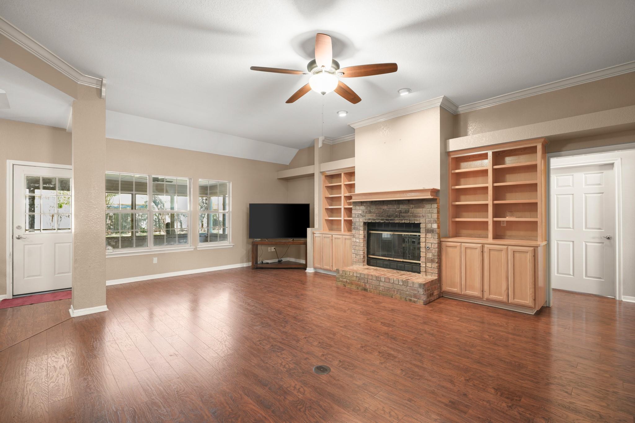
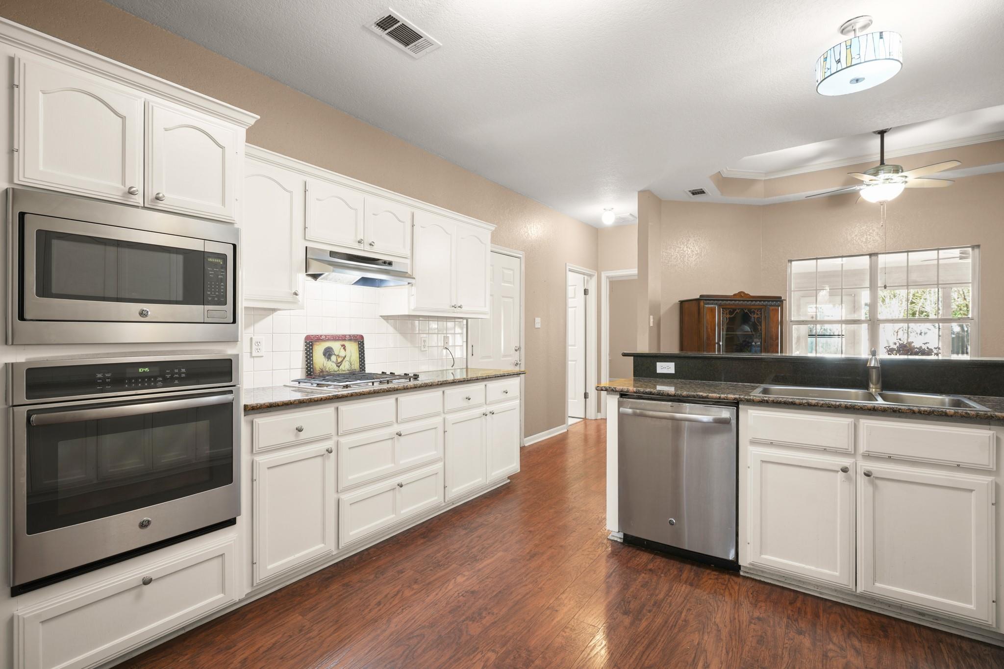
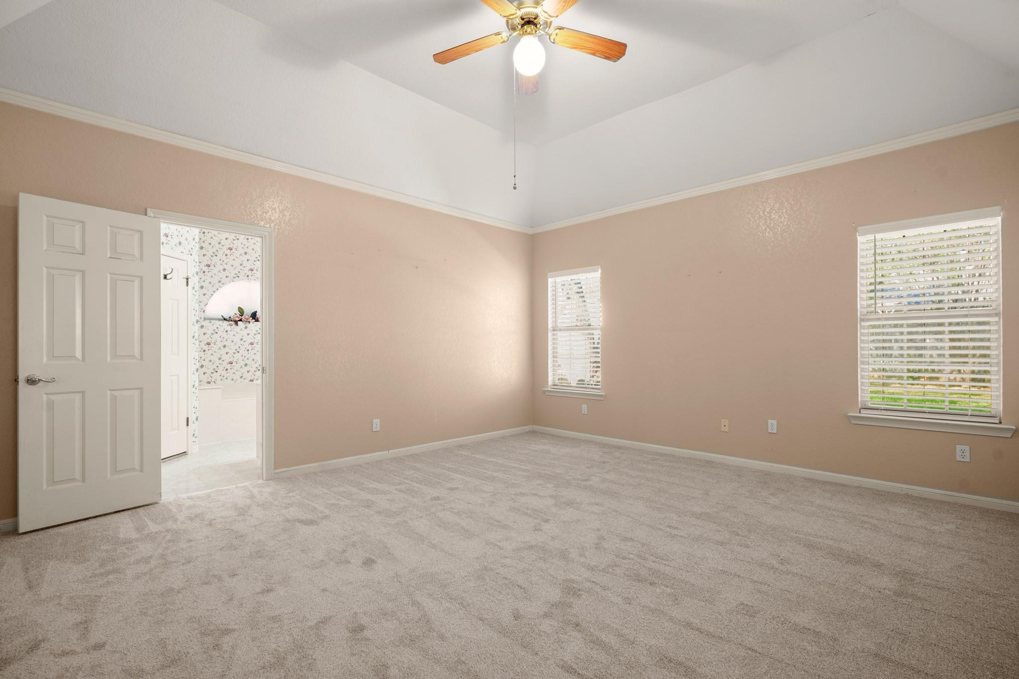
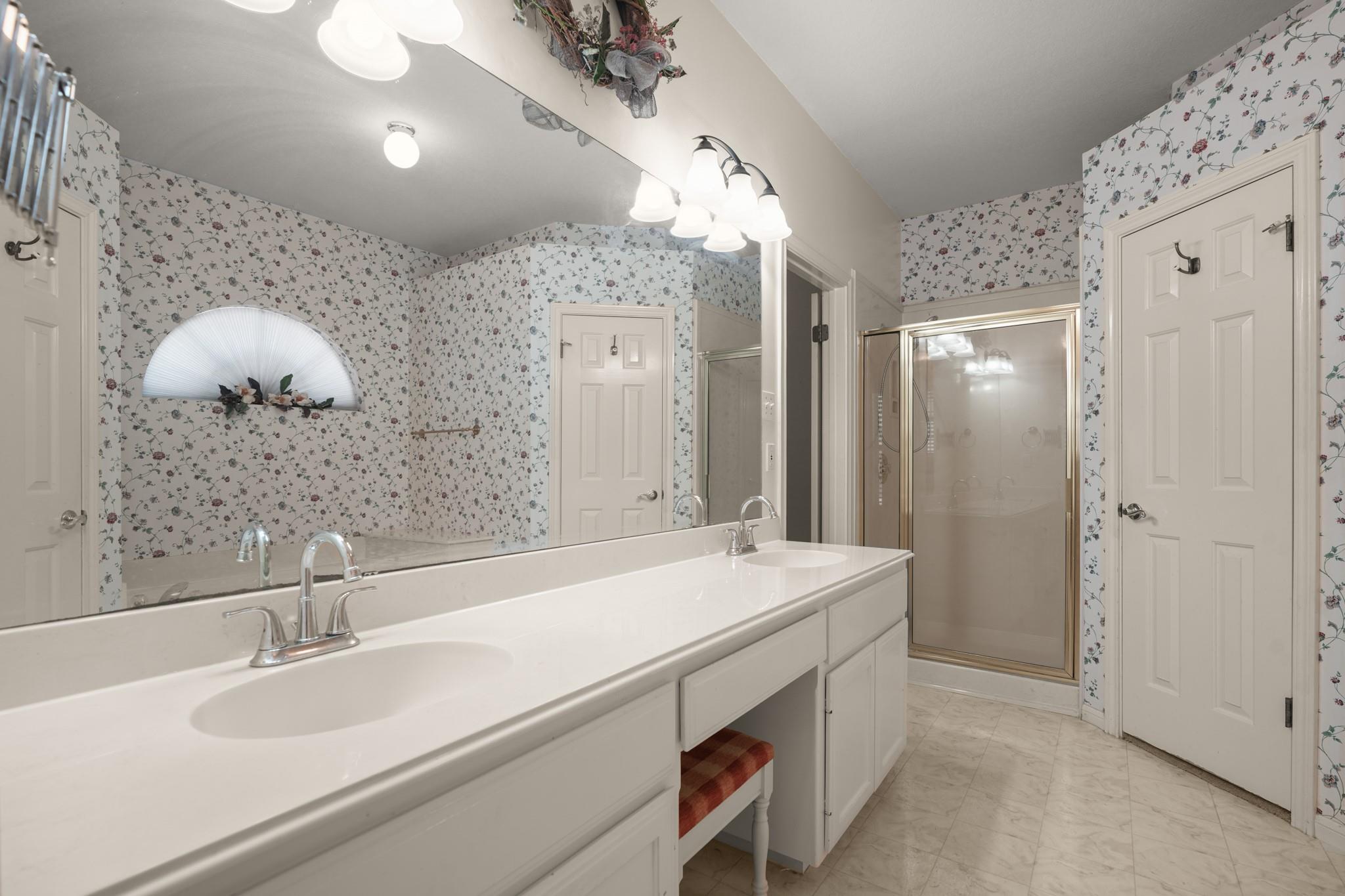
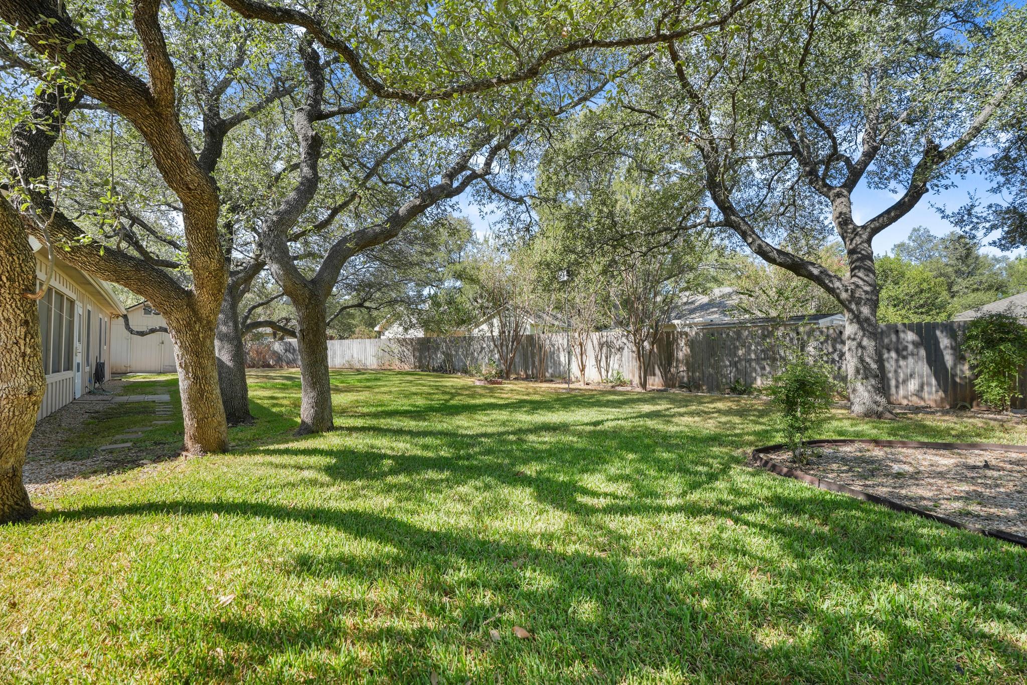
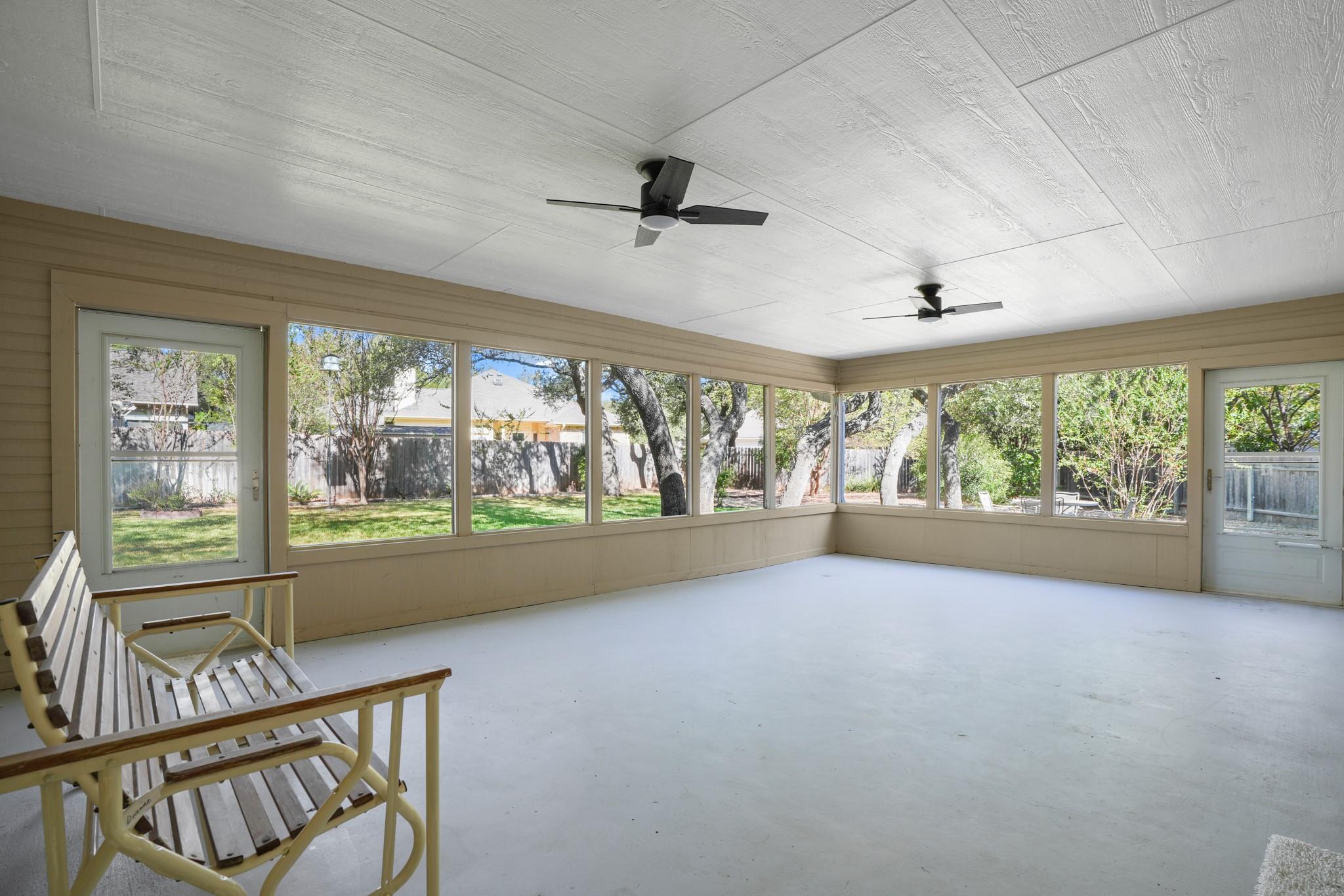
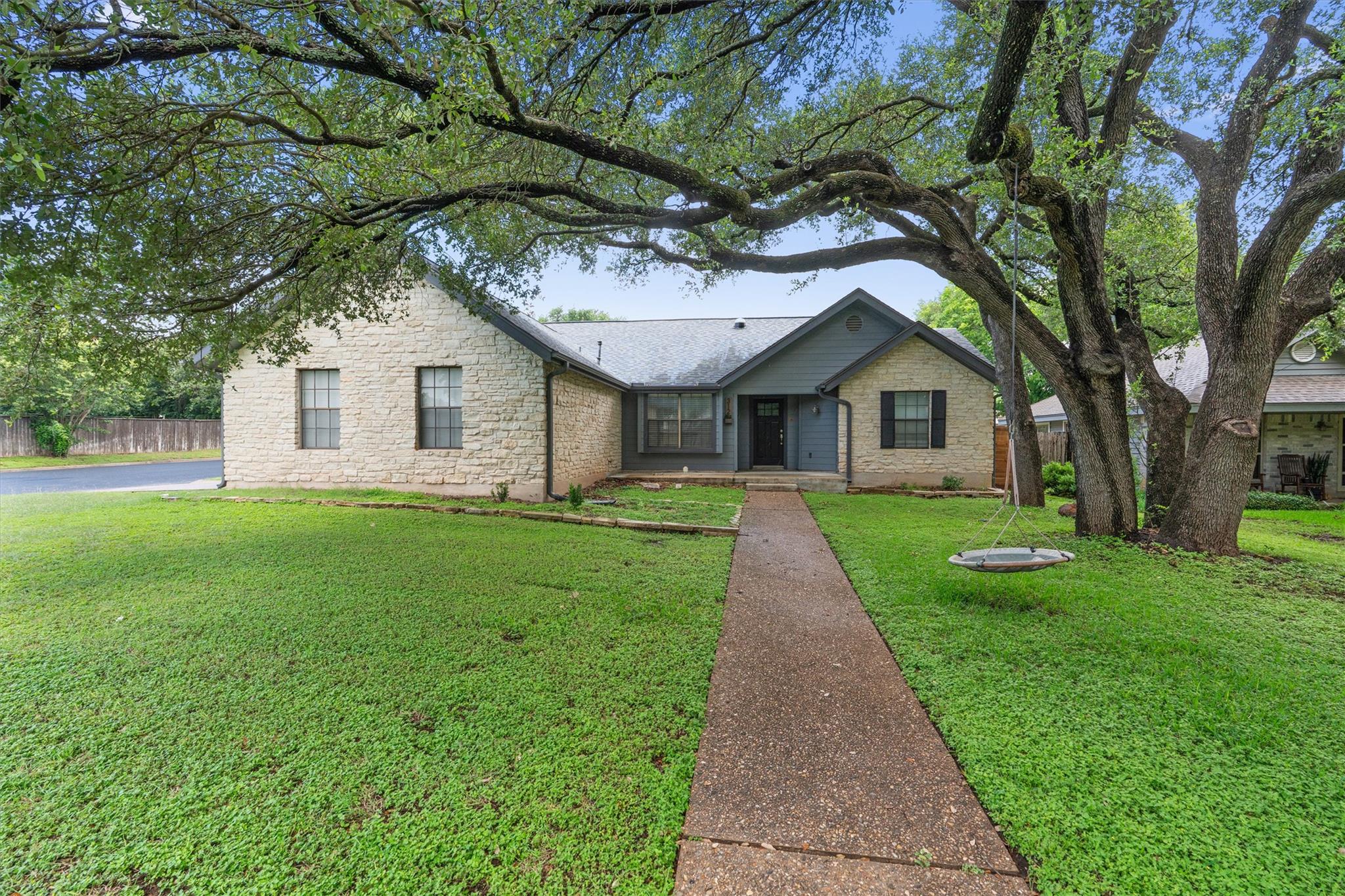
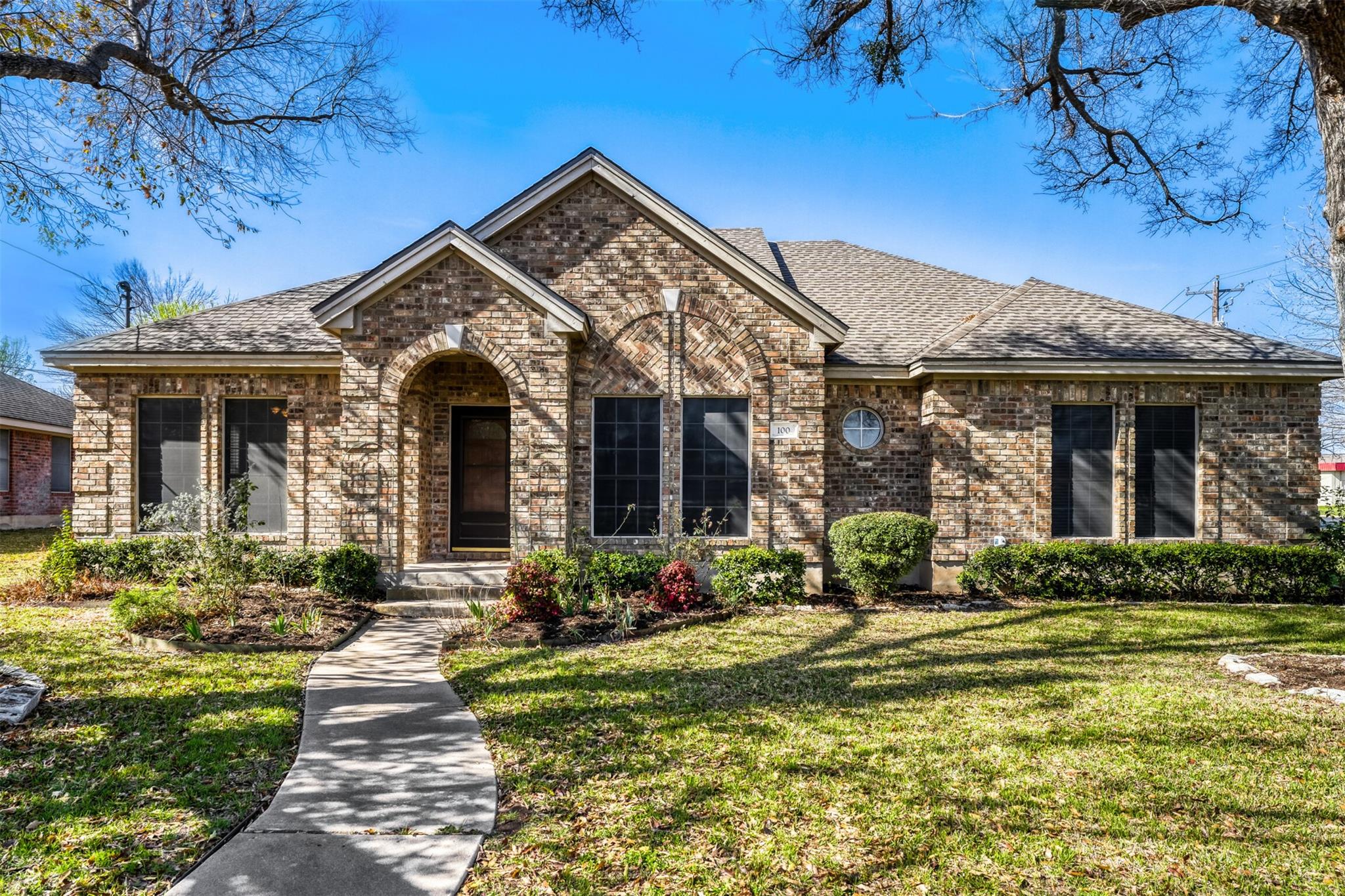
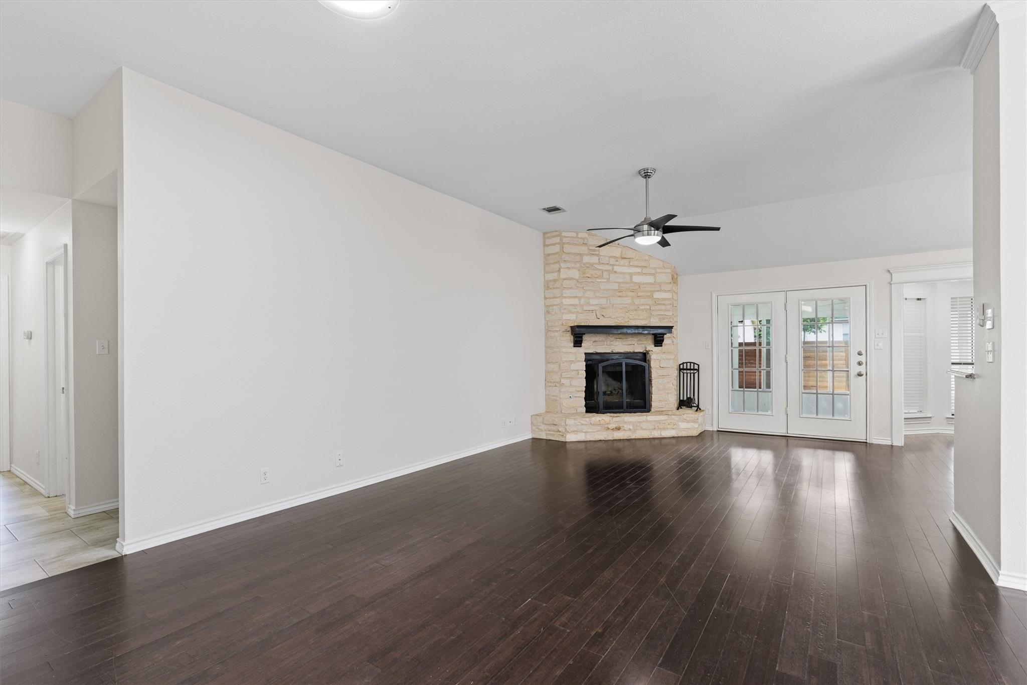
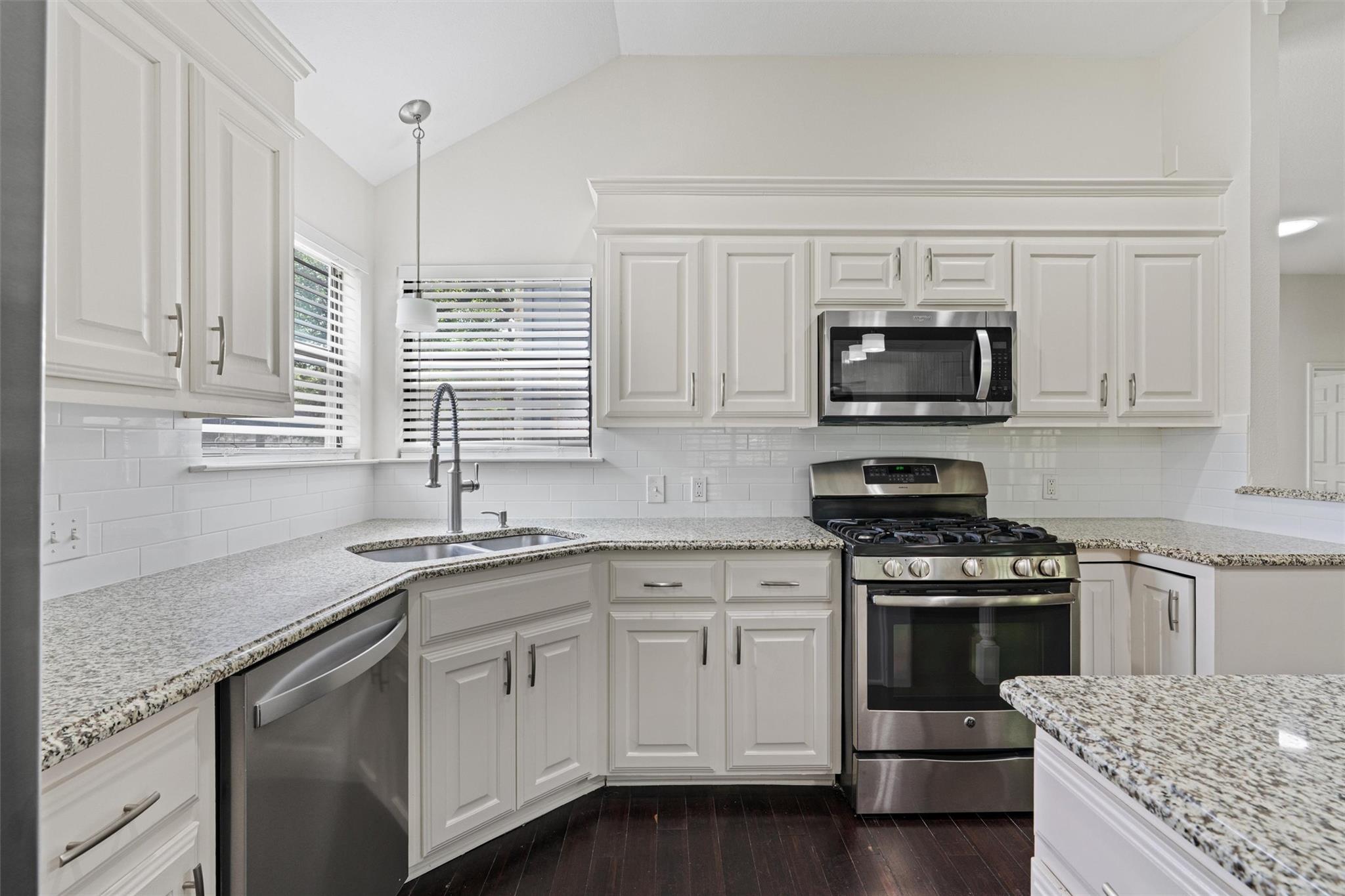
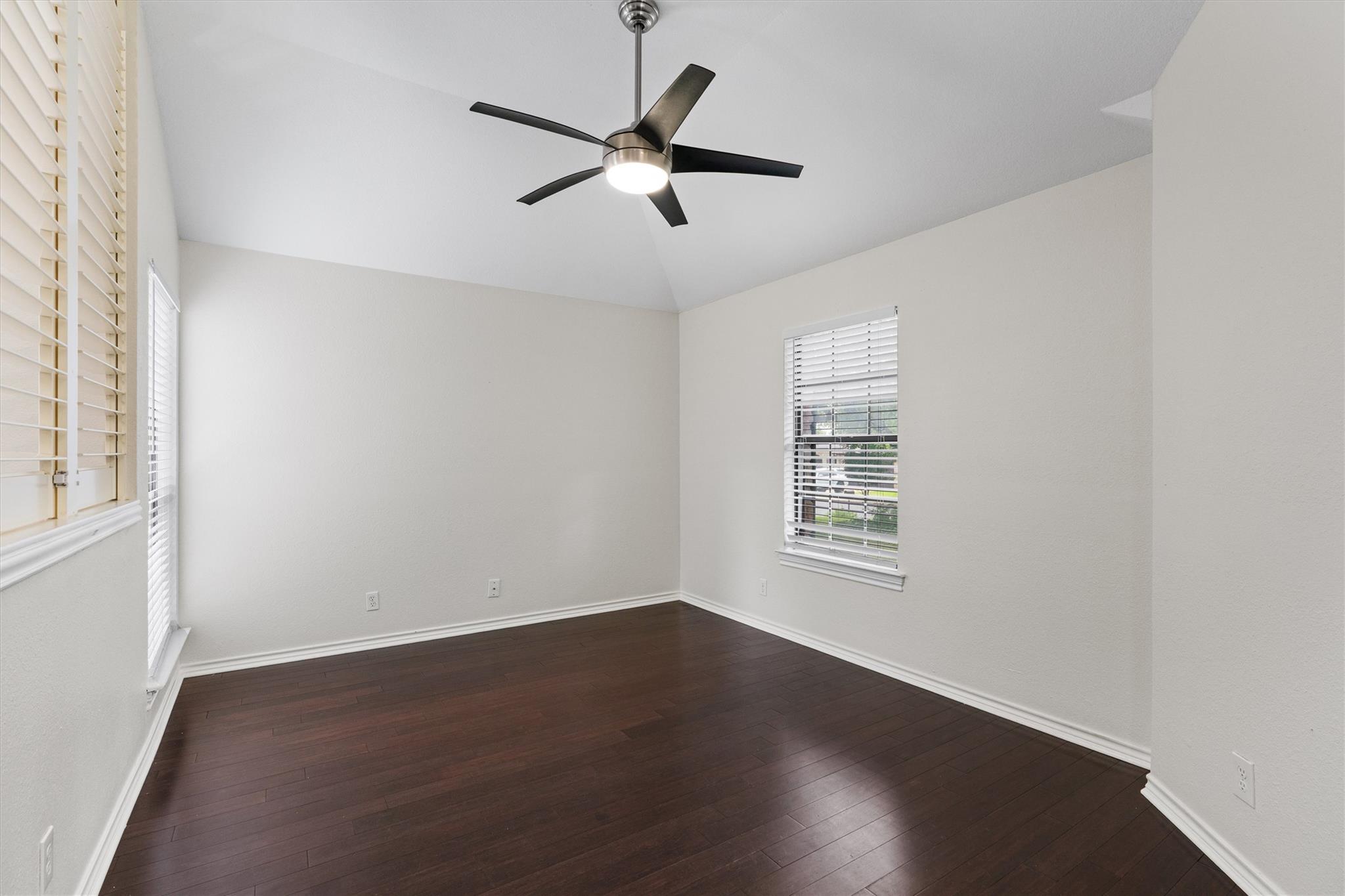
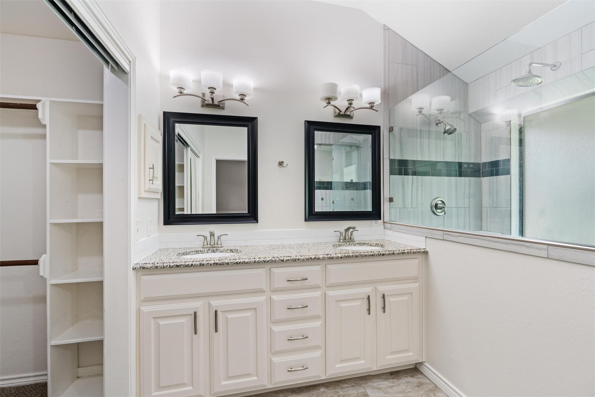
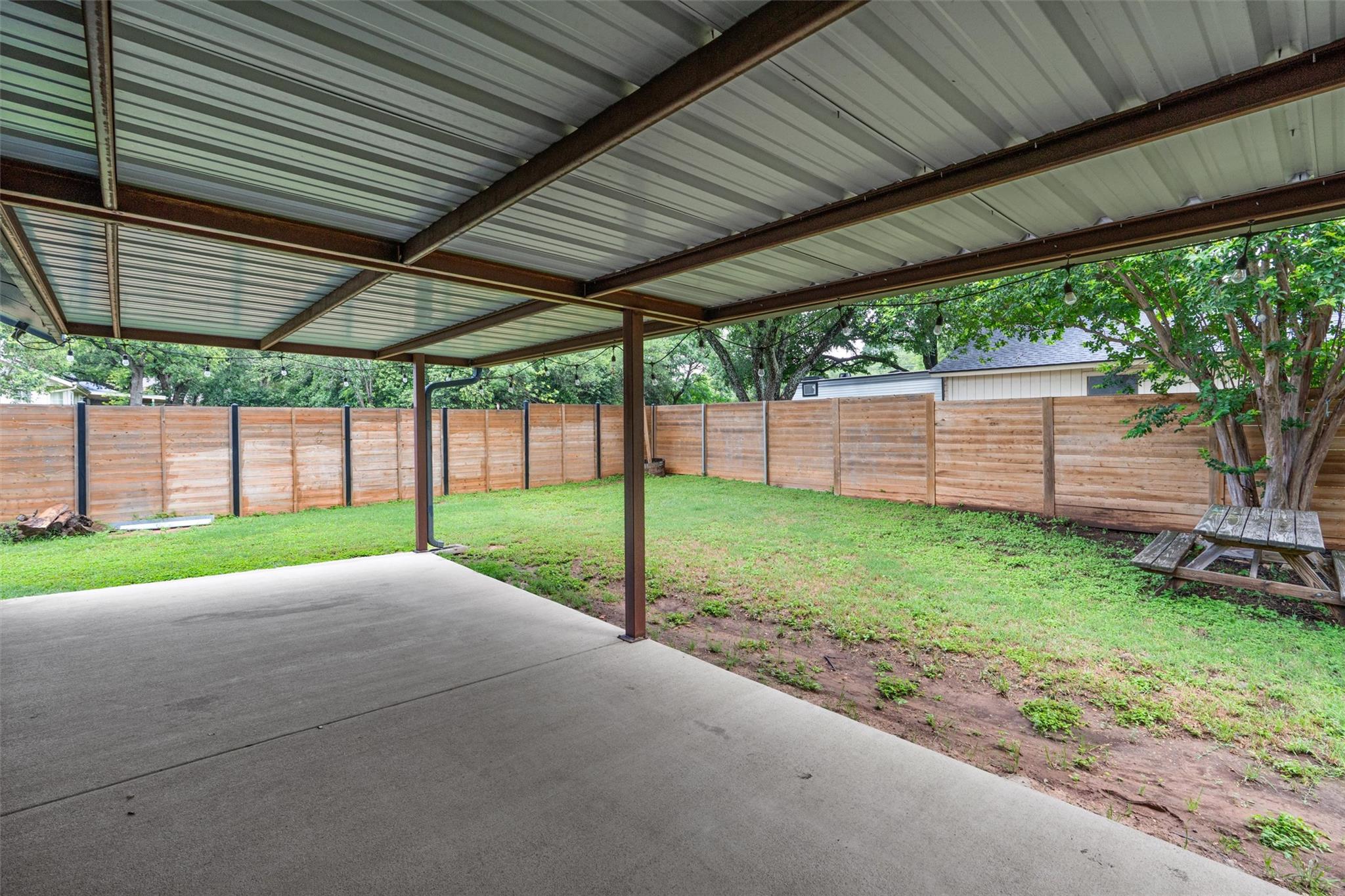
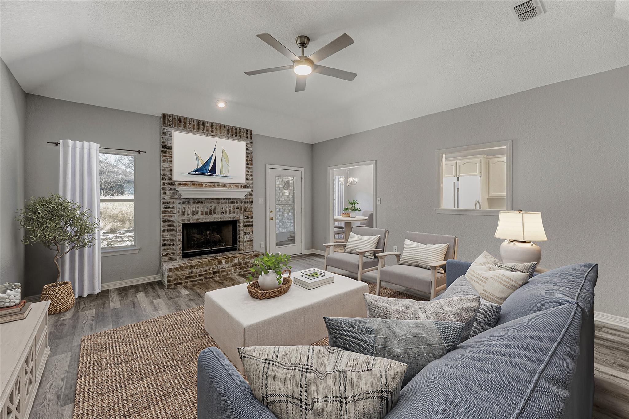
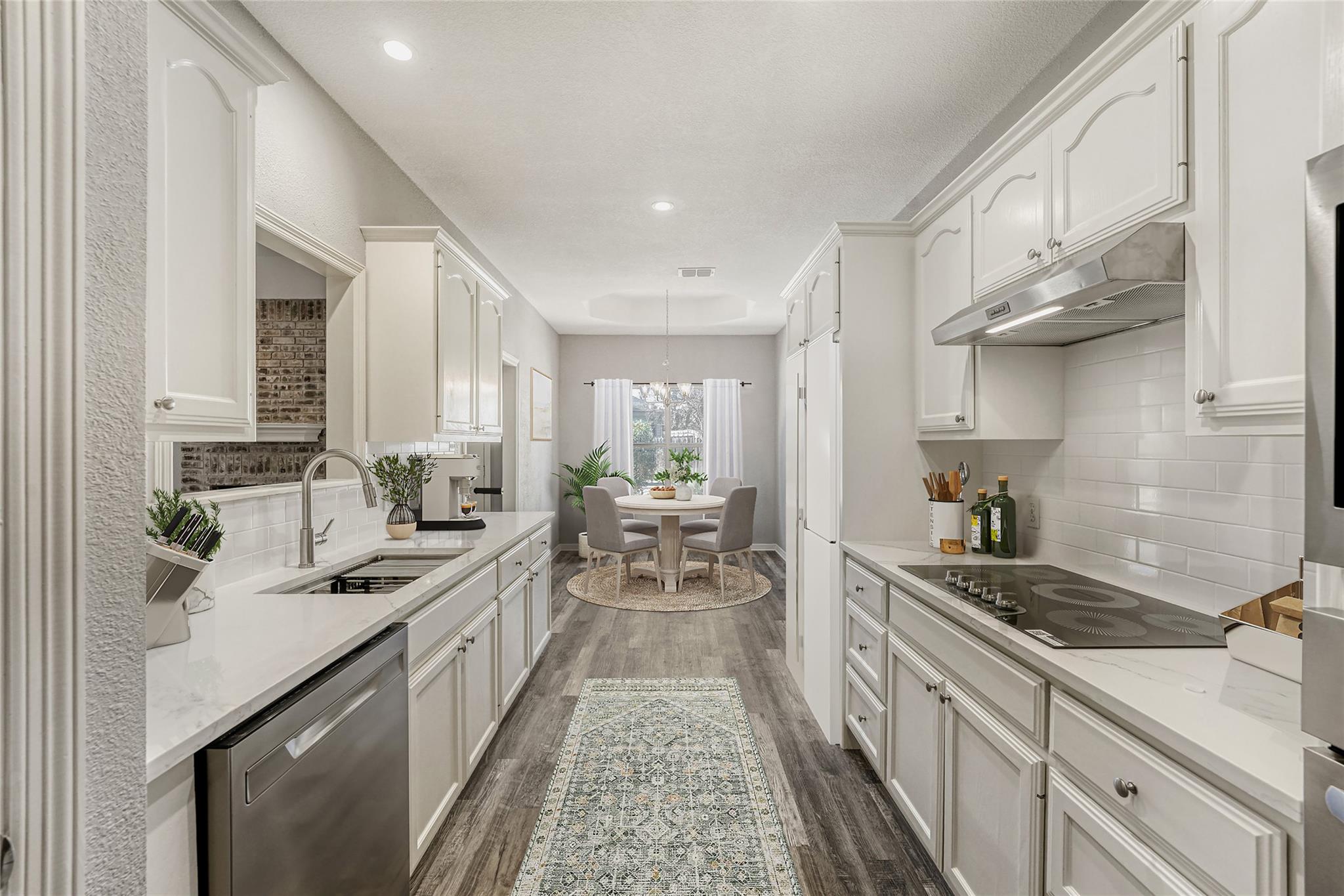
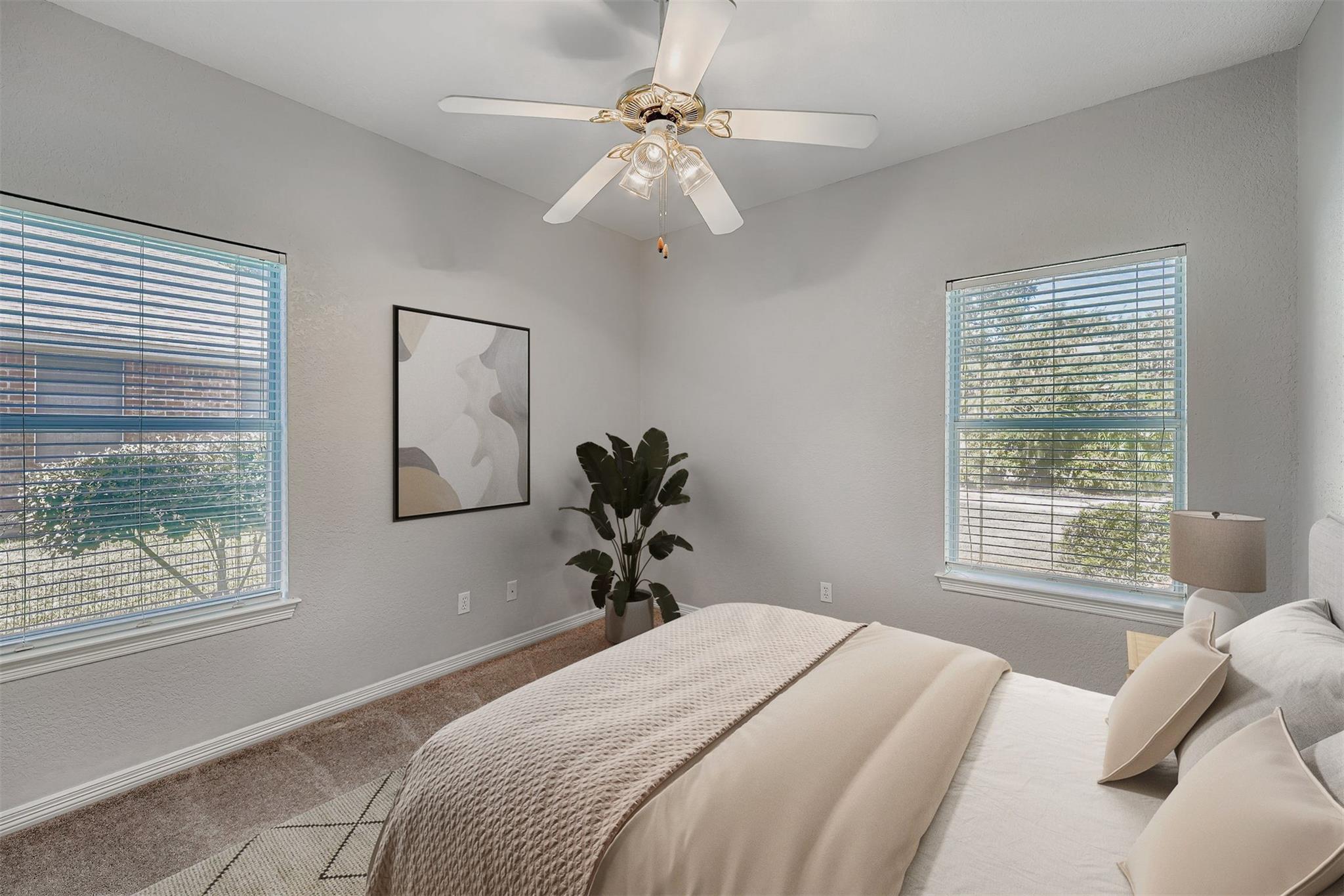
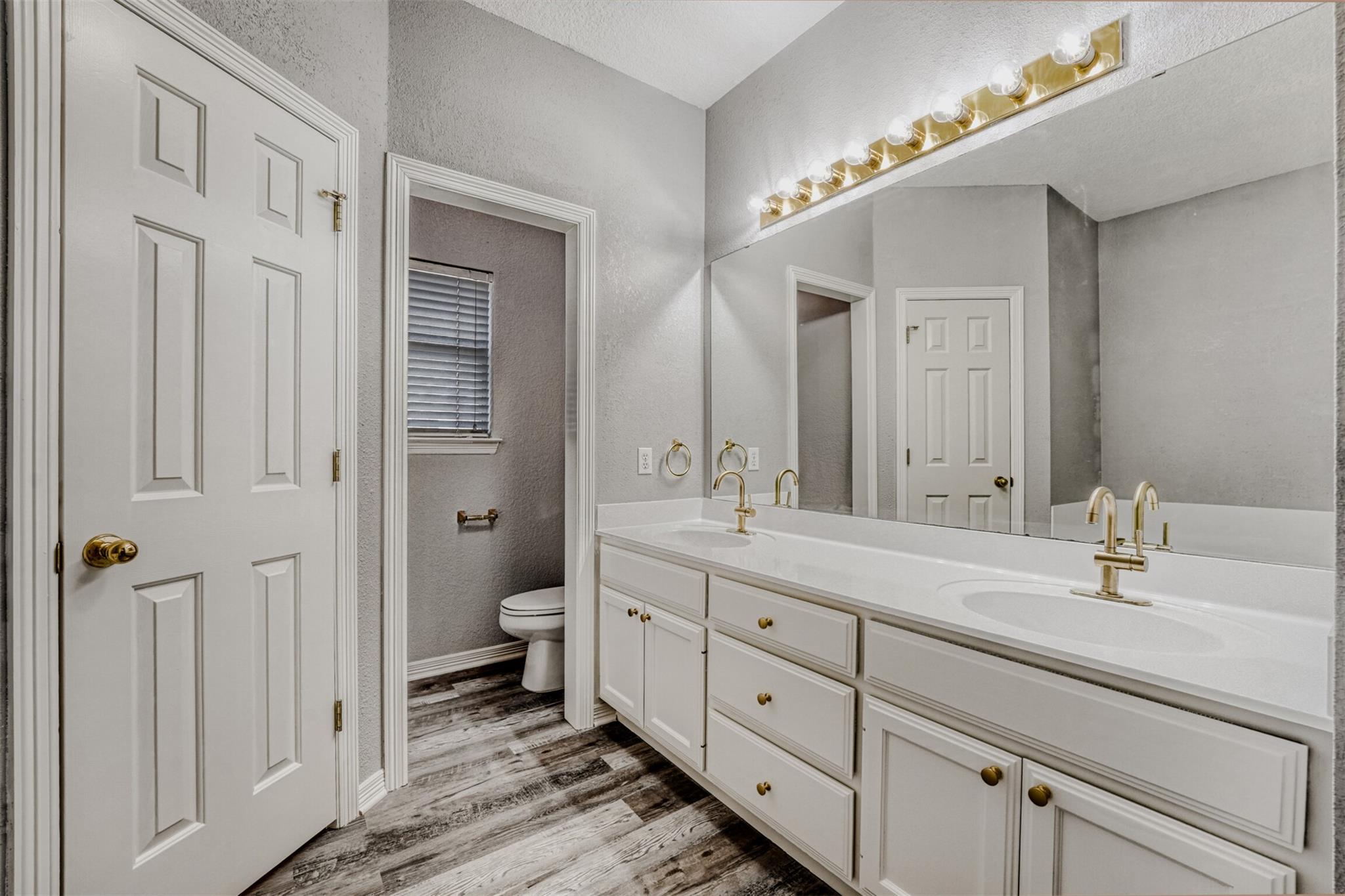
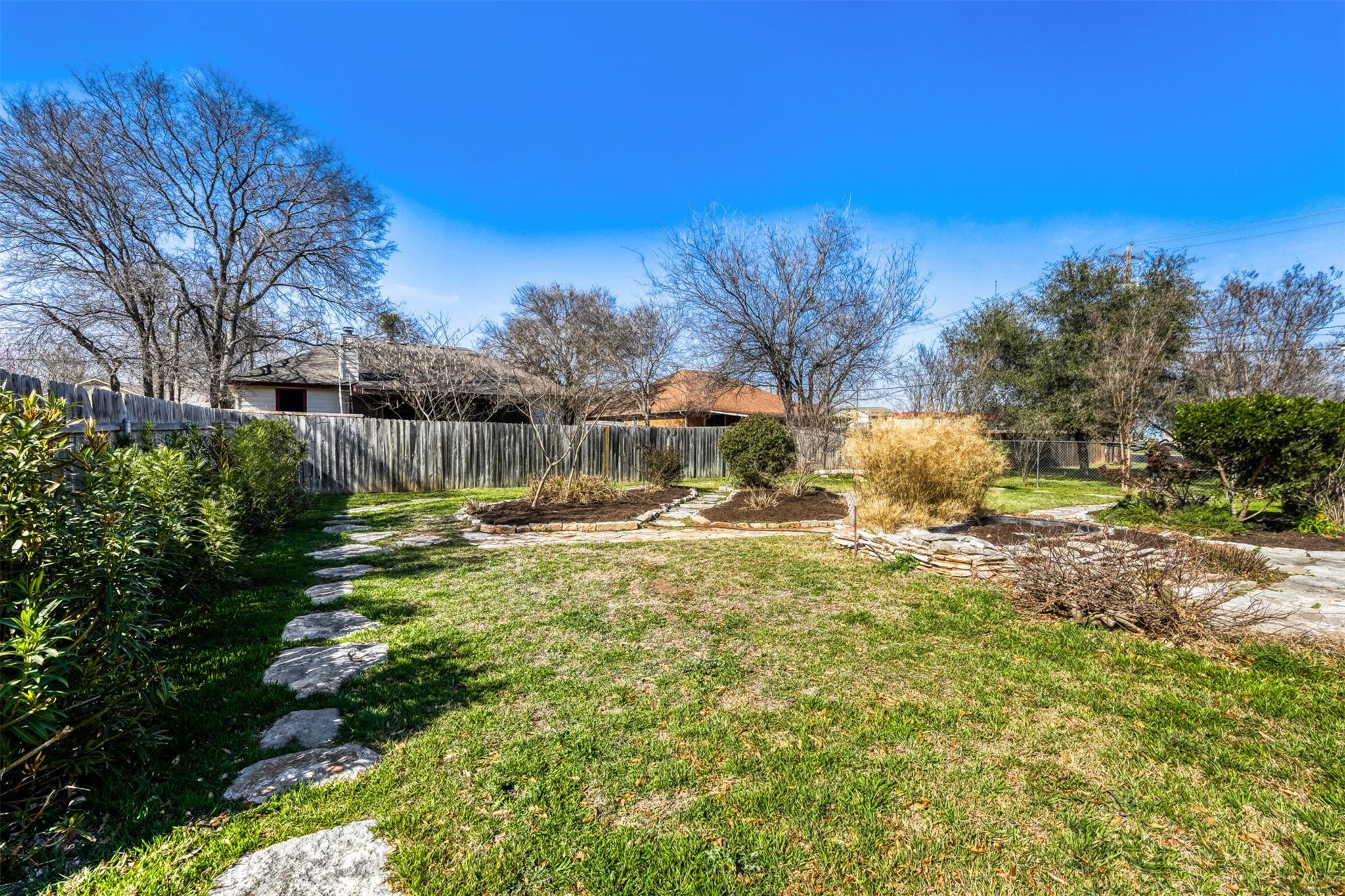
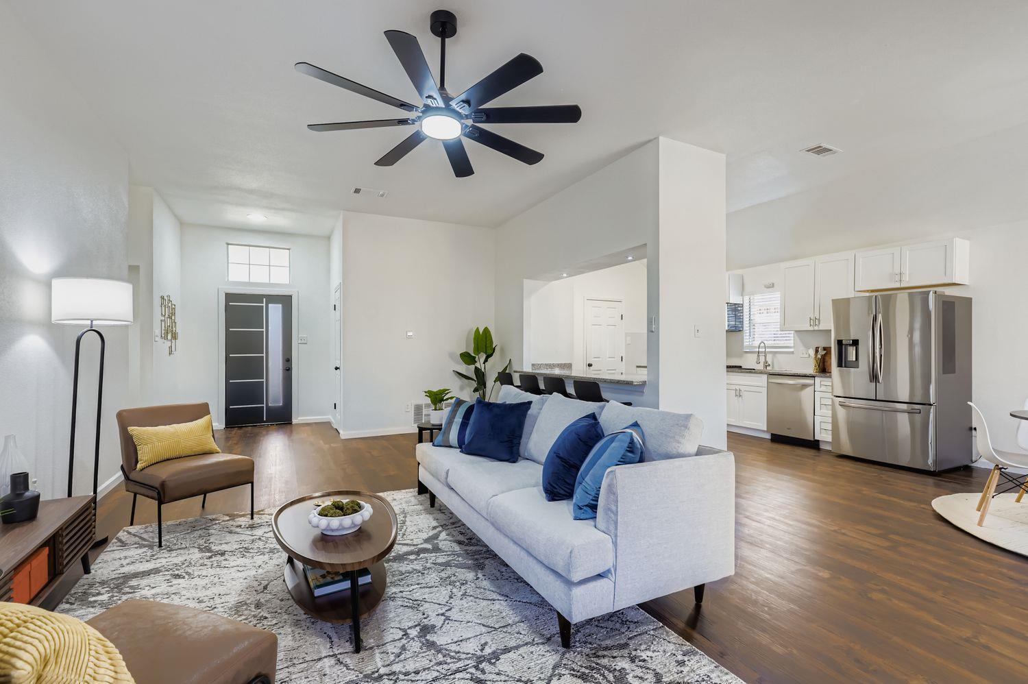
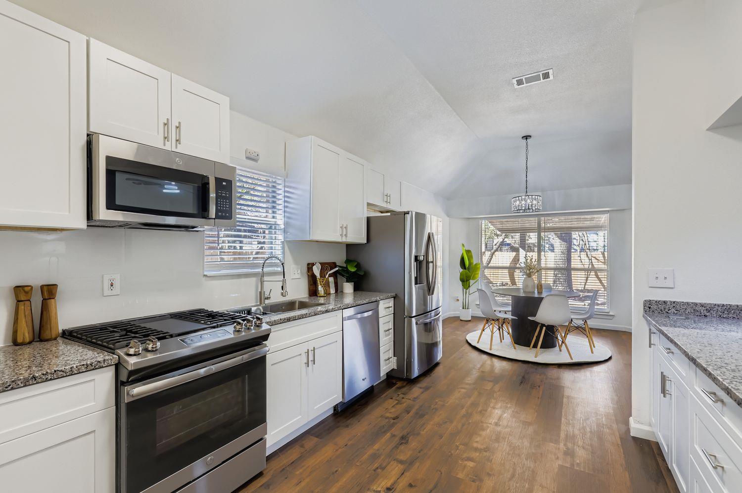
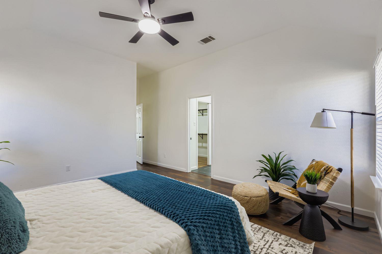
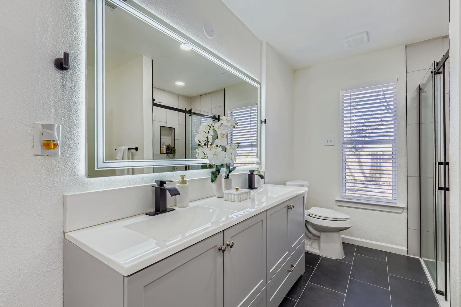
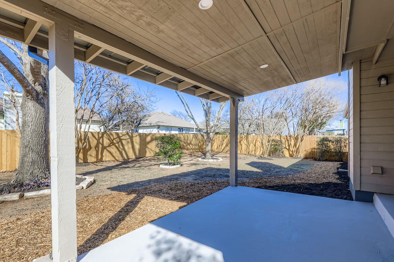
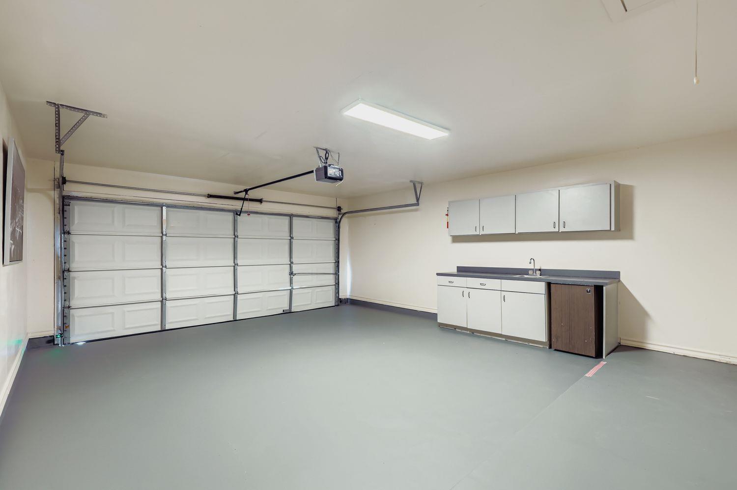
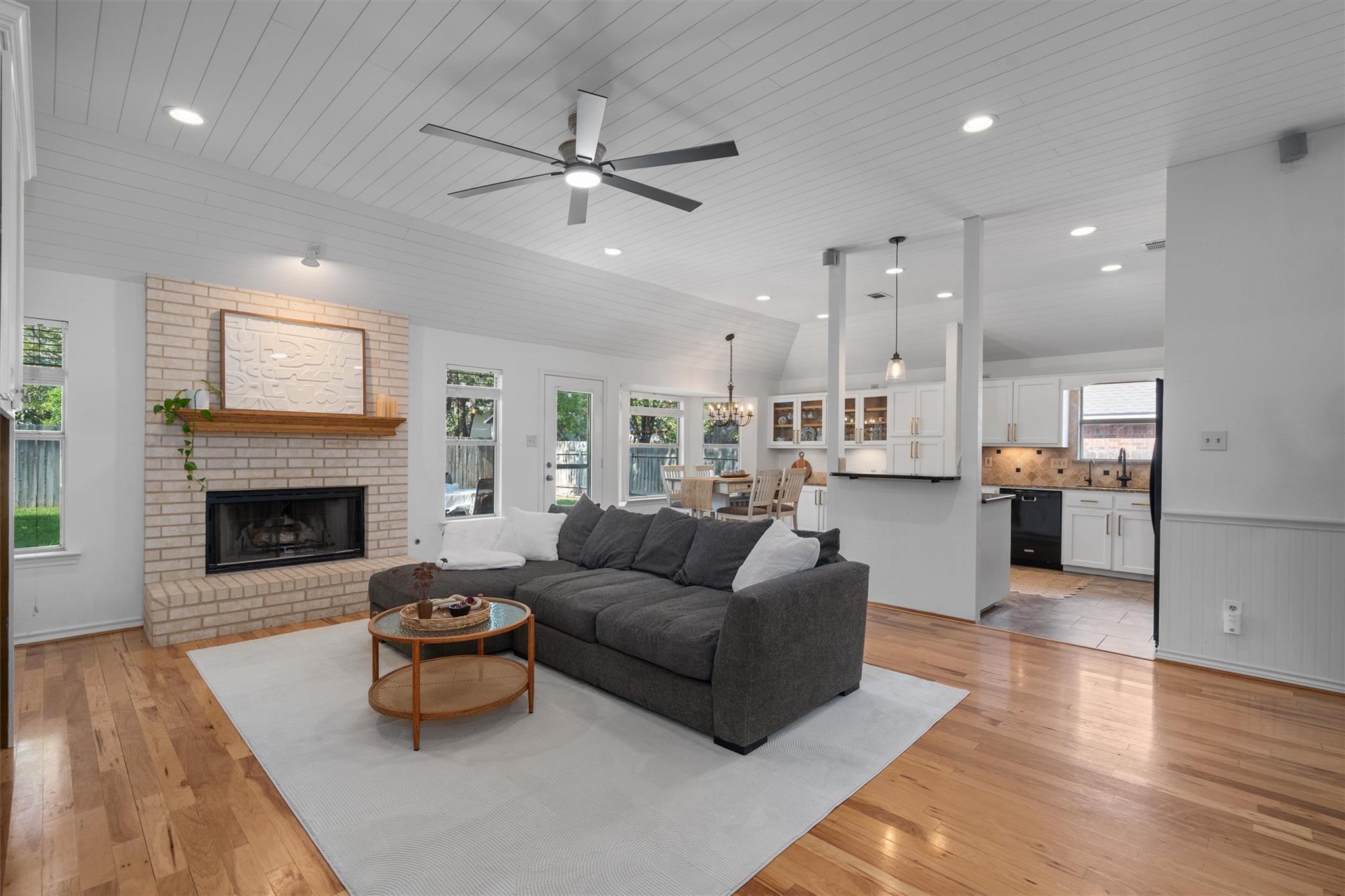
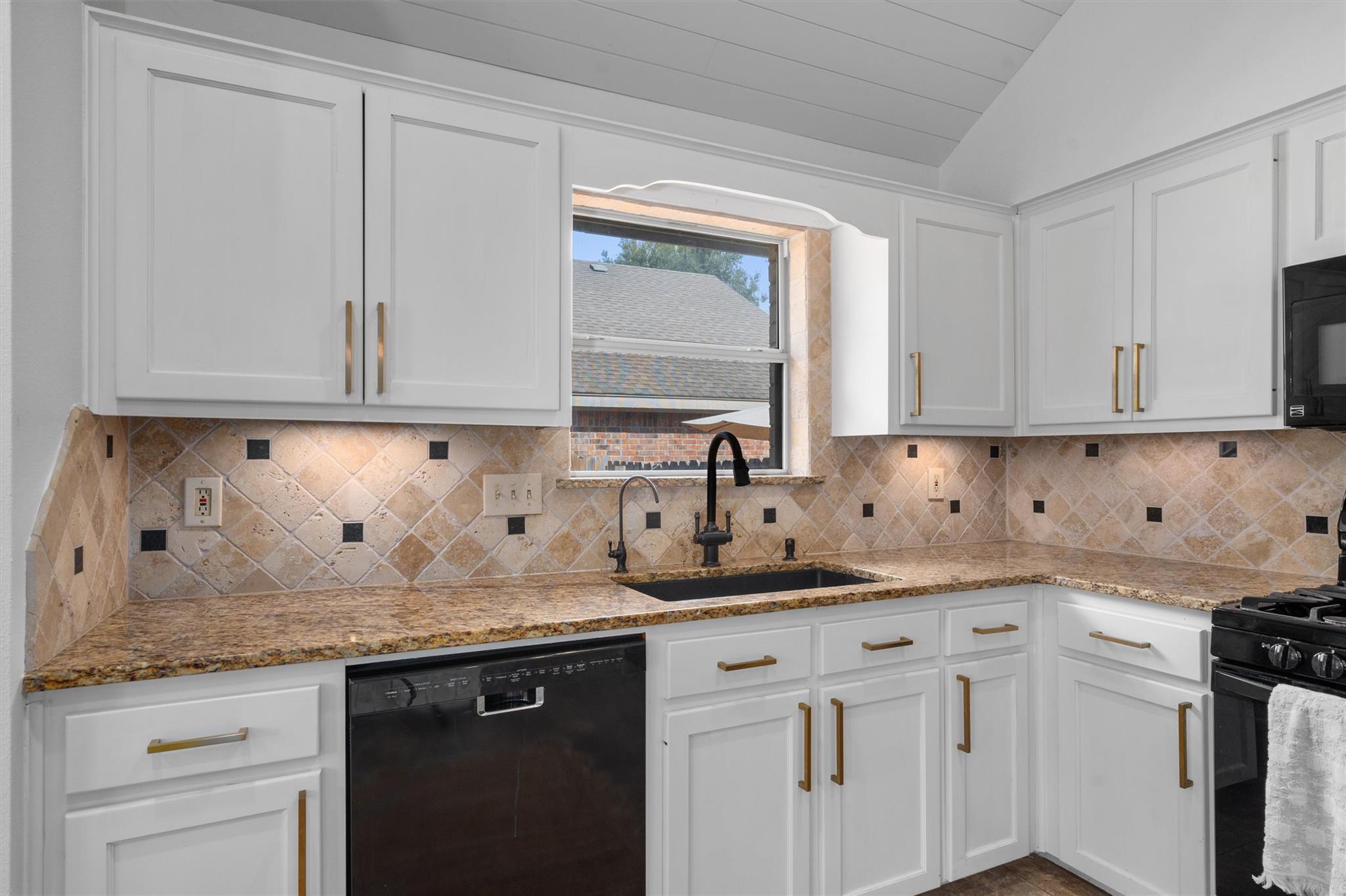
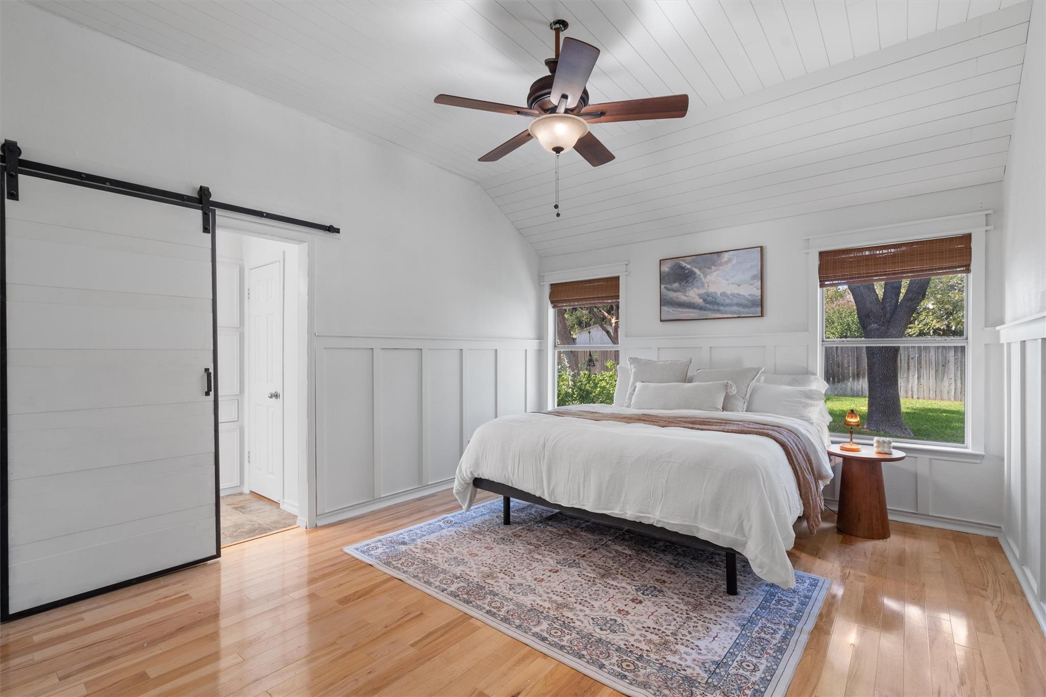
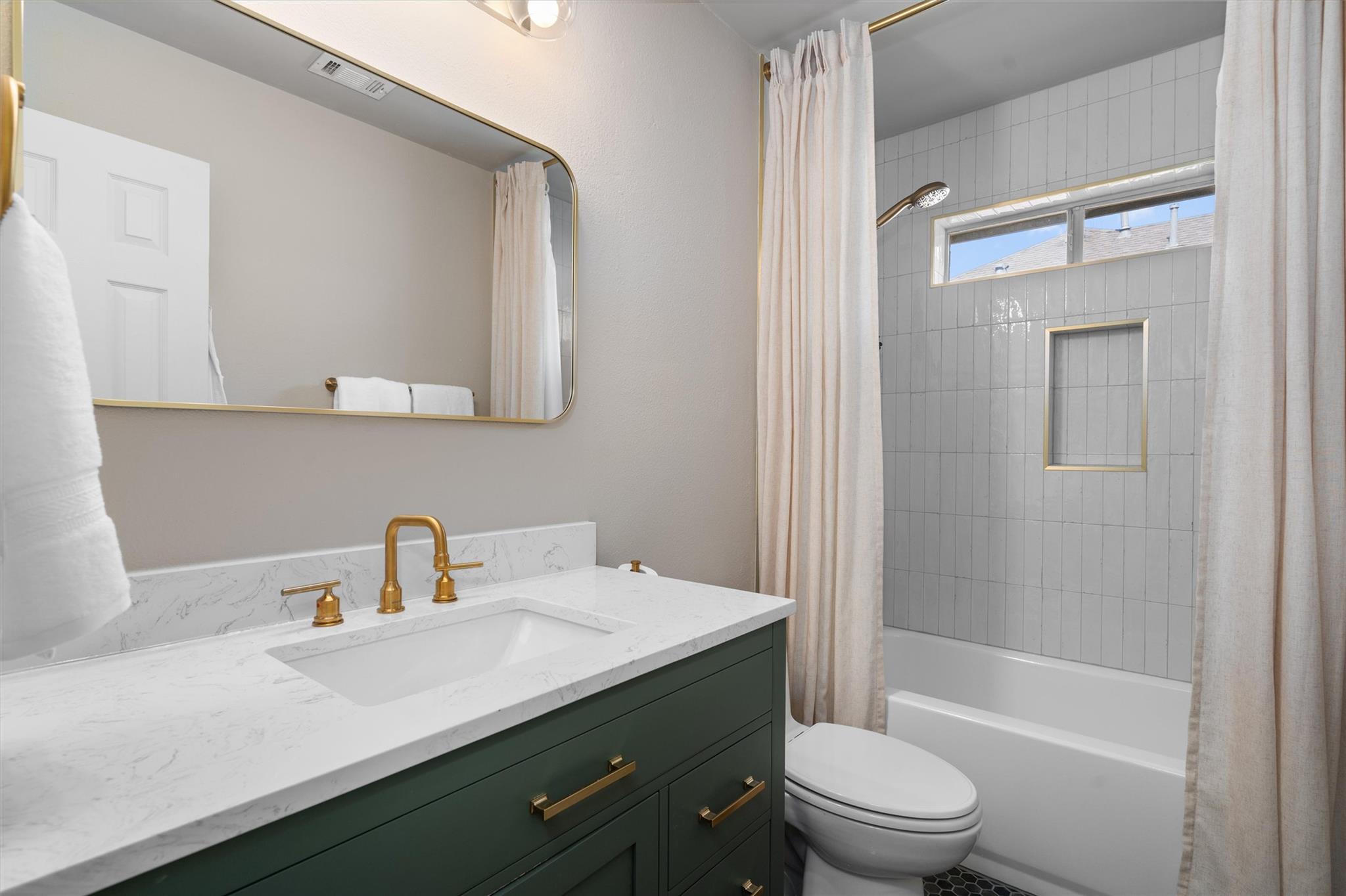
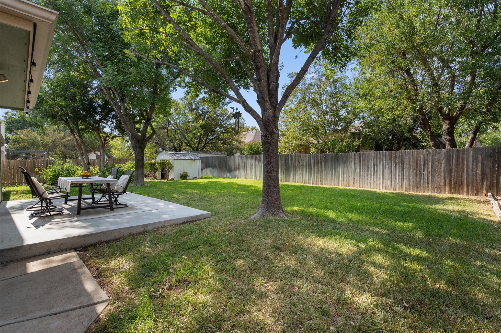
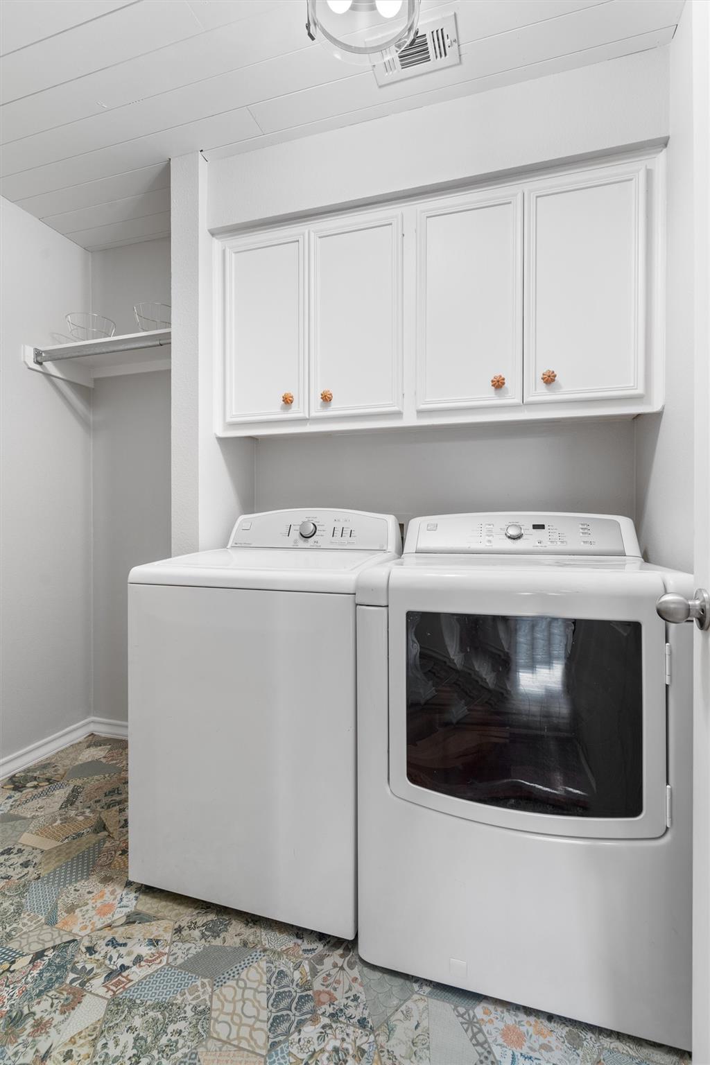
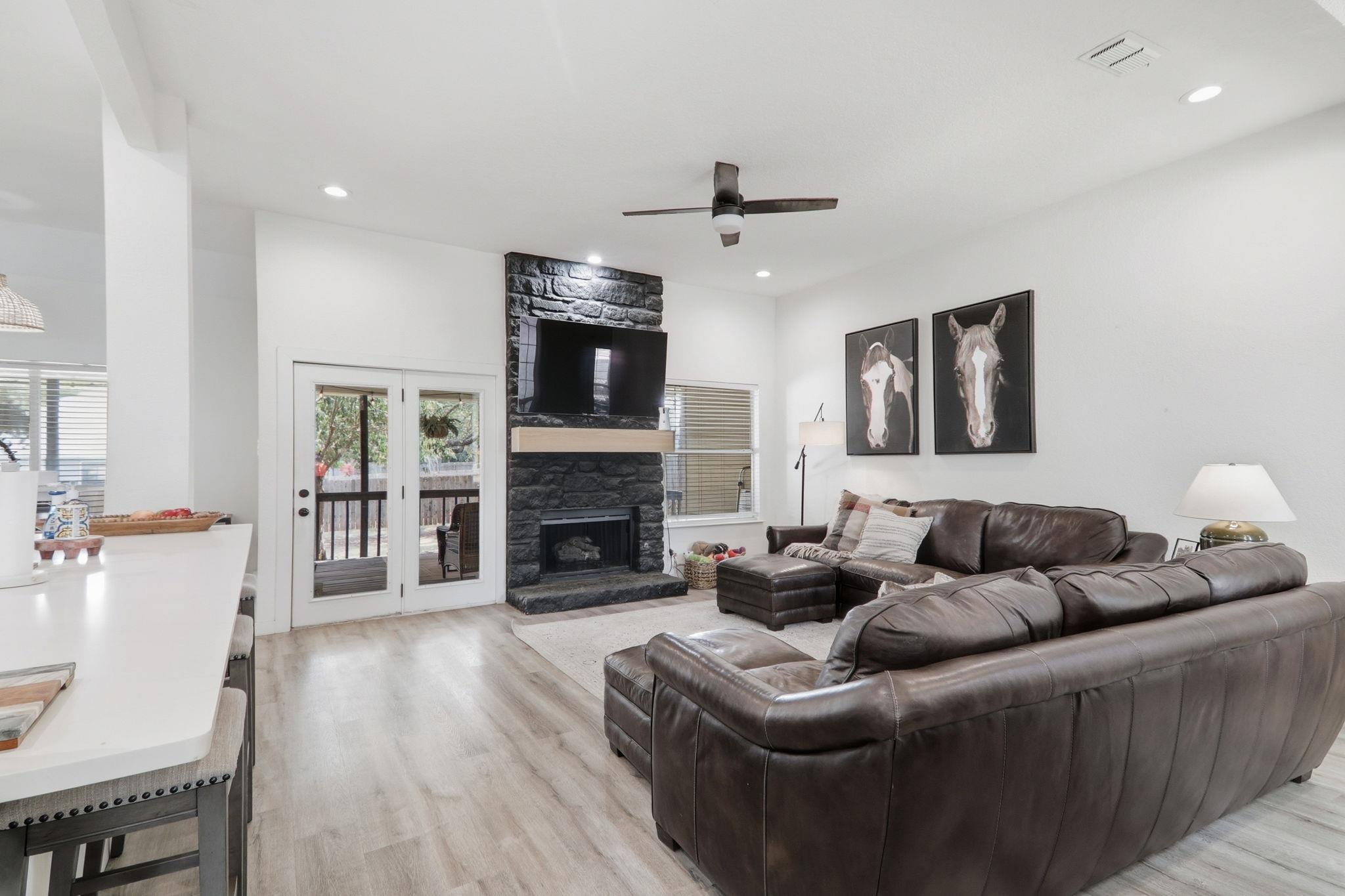
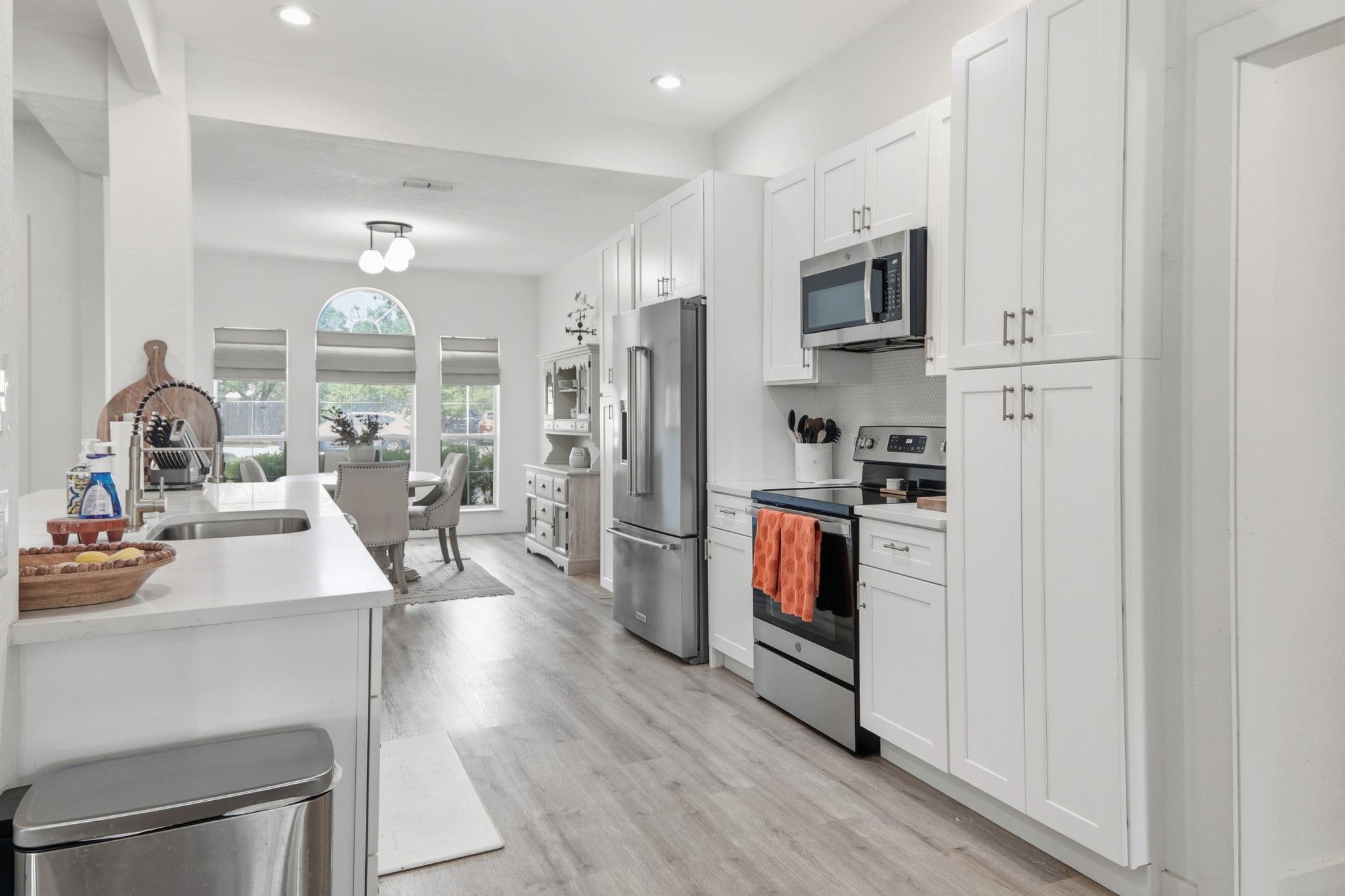
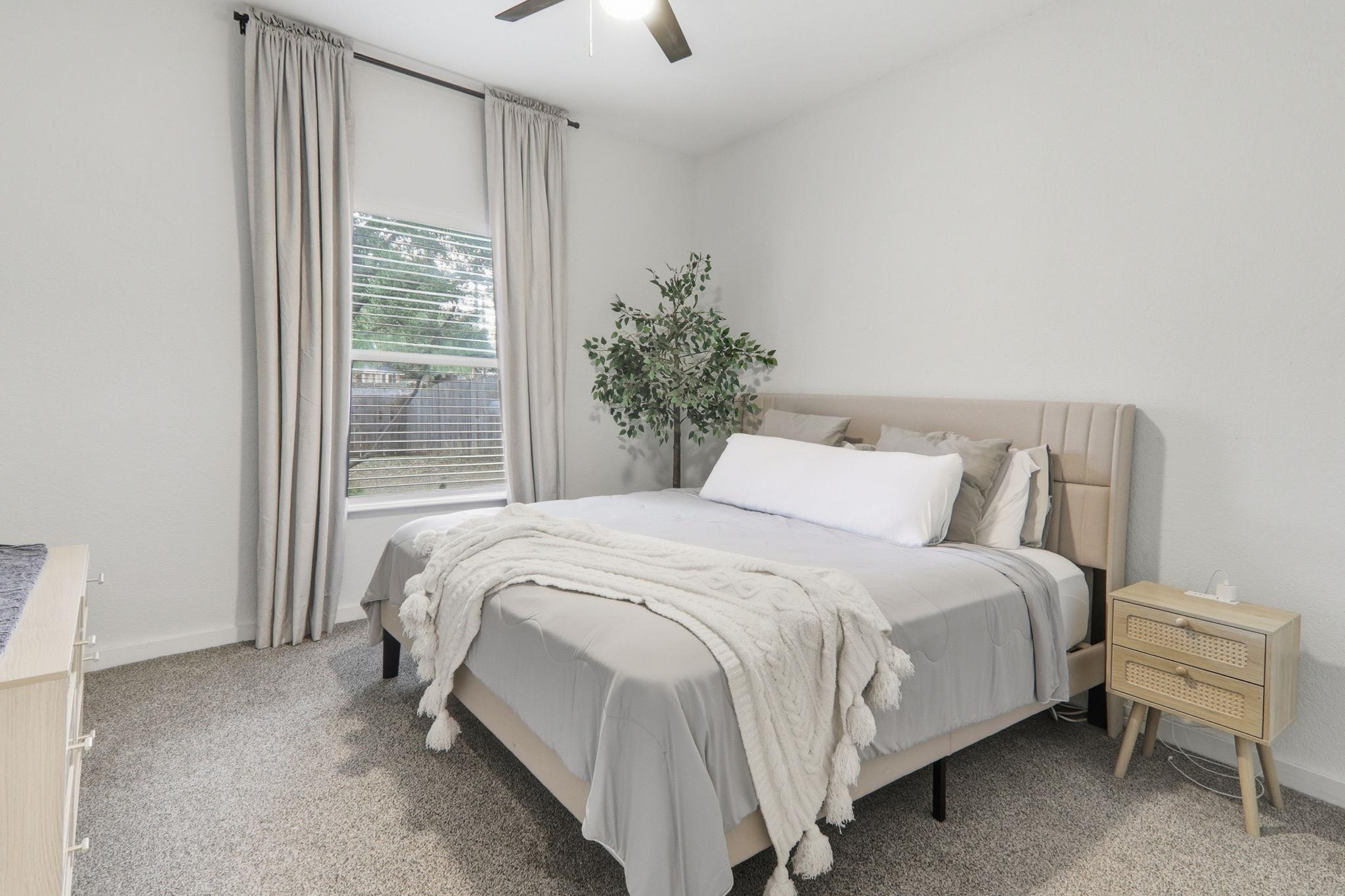
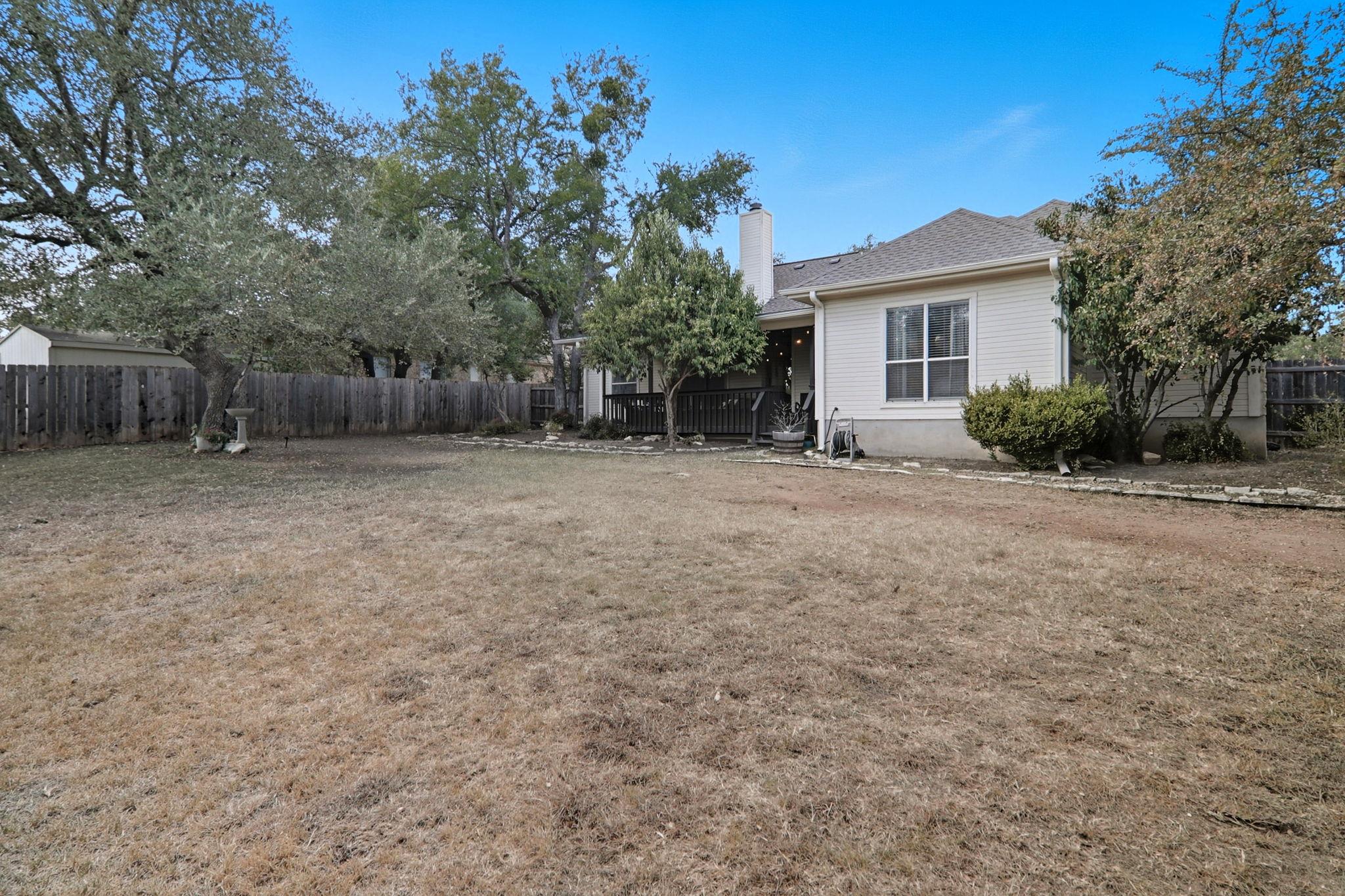
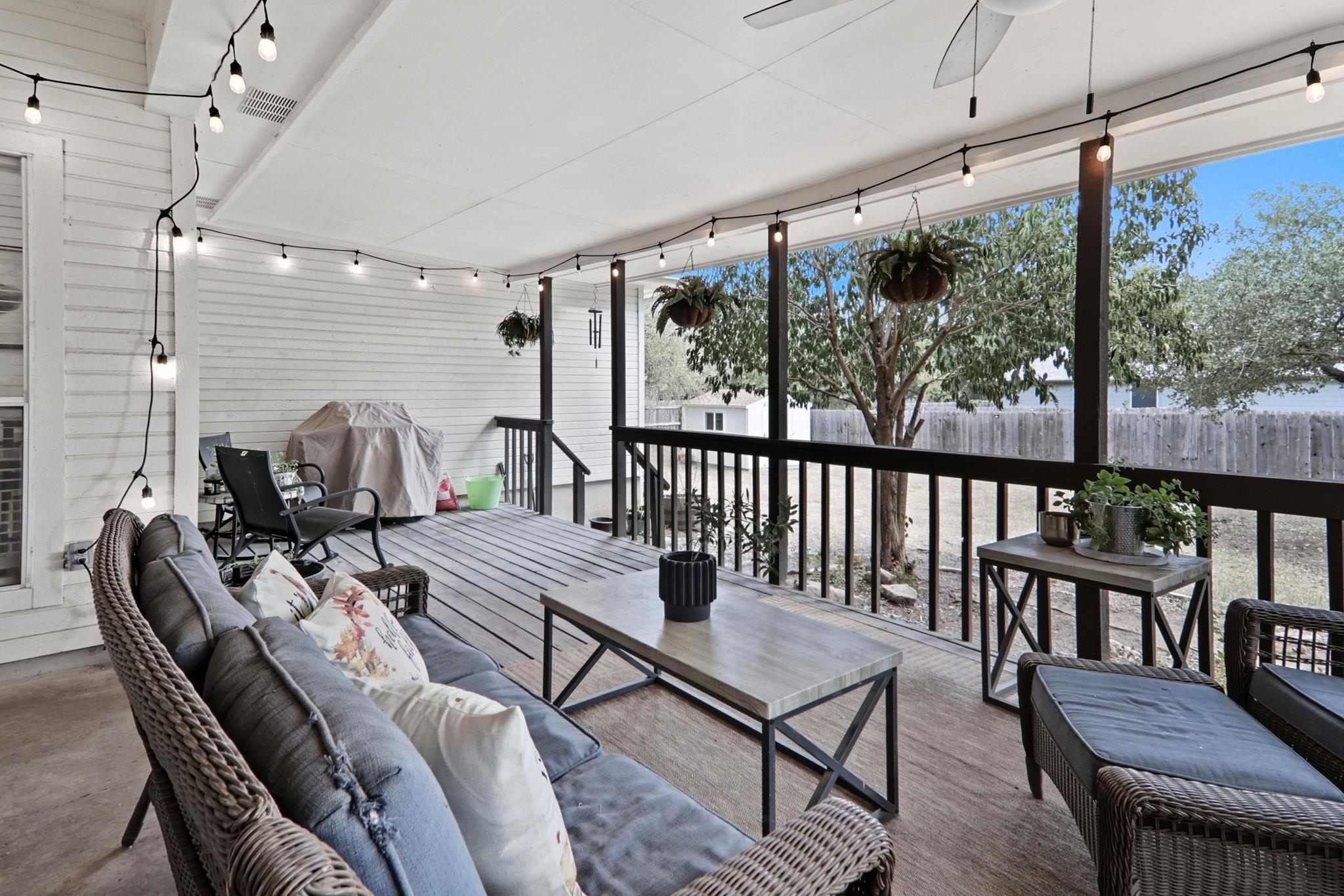
Living areaKitchenPrimary bedroomBathroomBack yardCovered patio
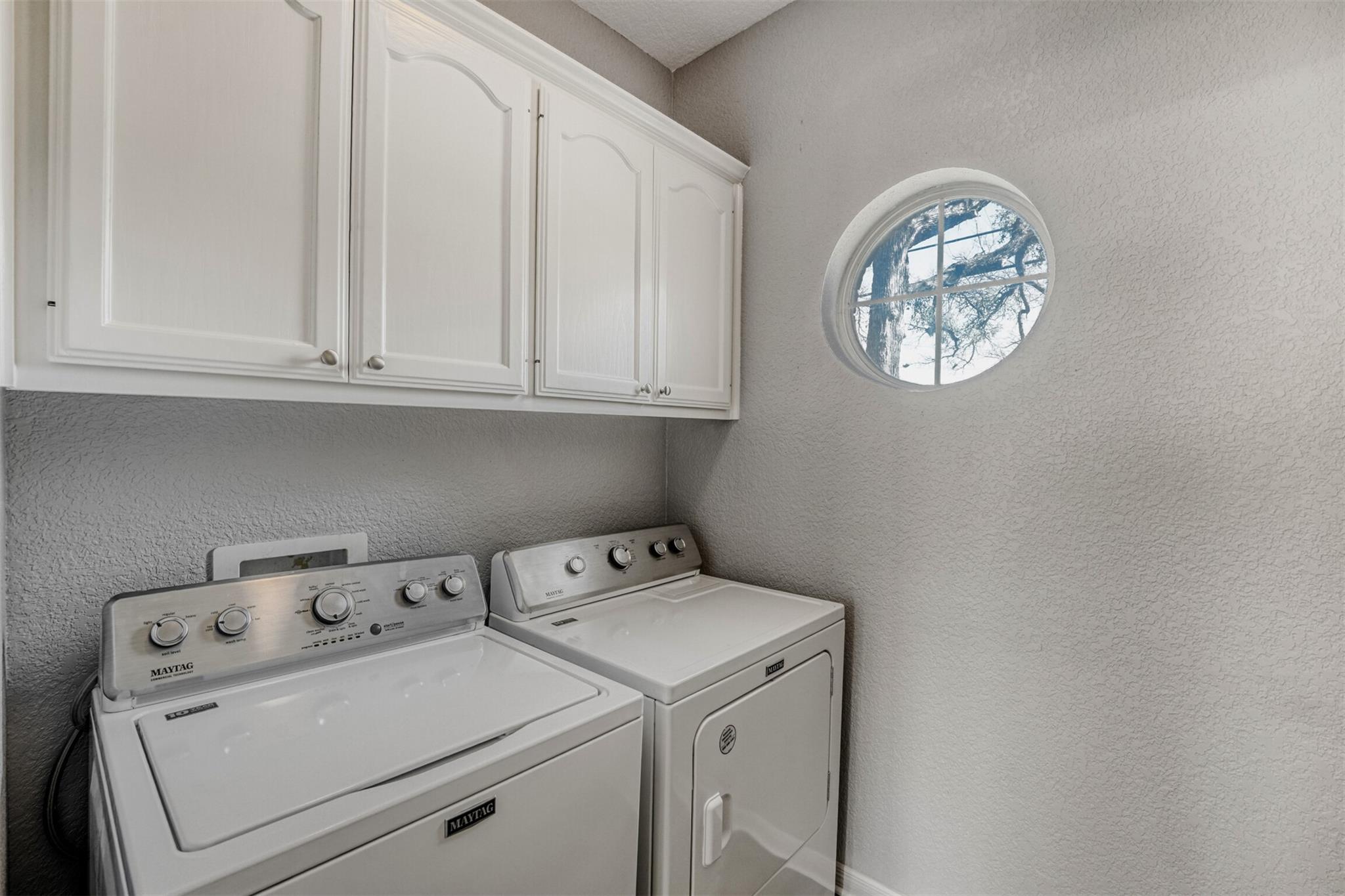
6 of the 24 photographs on this listing, chosen by ALEX Intelligence’s vision model — not from the MLS’s captions, which are generated. The 6 shown are the best examples of key property components that could be clearly identified.
Living area2,104 SFOne story
Bedrooms / baths4 / 2
Levels1
Garage2
Year built1992Older than most of Sierra Vista
Lot size0.40 ac17,437 SF
Days on market15Listed September 24, 2026
Williamson County 2026 market value$387,192WCAD total
Land value$82,500WCAD 2026
Improvement value$304,692WCAD 2026
Annual tax, as listed$7,0371.82% of the county market value.
Property details are from the Austin Board of REALTORS® MLS (ACTRIS) via Bridge Interactive. The market, land and improvement values are from Williamson Central Appraisal District. The annual tax is the figure reported on the listing.
Valuation
ALEX AI Statistical Model
Minimum$390,942
Average$417,312
Median$412,190
Maximum$450,753
ALEX’s statistical model uses five comparable sales. Each sale is
carried to this property’s 2,104 SF using the relationship between size and price
per SF that the model measures from these sales. Each sale is then weighted by how
closely it resembles this house on six measured characteristics.
Traditional Arithmetic Model
Minimum$407,593511 Debora Dr
Average$448,080
Median$450,262
Maximum$484,299104 Susana Dr
The same five sales, each counted equally and without the size
carry. How the two rows differ is explained below.
Click here for details
In plain terms
Sales that are more like
this property — closer in size, age, lot size, room count and distance, and more
recent — count for more, and the way price per SF changes with size is
measured from the sales themselves rather than assumed.
What the method is called
Comparables are chosen by Mahalanobis-metric nearest-neighbor matching with
calipers (a caliper is a maximum allowed difference), and the valuation
is a kernel-weighted local linear regression — a local polynomial
fit, the same family as LOESS — evaluated at this property. Both run inside
ALEX’s valuation engine.
Which sales are admitted, and the boundary that is not drawn
The search starts as close to this property as the market allows. It tries the same
street within its subdivision, then the same phase or section, then the subdivision
family (every section and spelling of its name in this city, treated as one place). Only
when the tighter area holds too few usable sales does it widen, to rings of half a mile out
to five miles, and then to the ZIP code. It is not capped at
the subdivision. A hard boundary sounds safer than it is: where a subdivision has produced
four sales in two years, confining the model to them buys a tidy boundary at the cost of
a valuation resting on four houses. Where the pool does widen, every rule that widened
it is printed in this report, with how many sales each step admitted or dropped.
How far apart two houses are
Similarity is not distance on a map. Each sale is described by six measurements:
living area in logs, year built, lot size in logs, distance from this property, months
since it closed, and bedrooms plus half the bathrooms. The Mahalanobis
distance combines all six into one number, scaled by how much each varies in this
market and, where the market area holds enough sales to measure it, corrected for the
fact that they move together. Bigger houses tend to be newer and to sit on different
lots; a plain straight-line (Euclidean) distance would count what is largely one
difference several times over. Geography is one of the six, not the whole of it — a
near-identical house half a mile away is better evidence than a different house across
the street, and the metric says so.
The kernel, and why this one
Each admitted sale is weighted by an Epanechnikov kernel of its
distance: with u = d/h for bandwidth h,
the weight is 1 − u², reaching zero at the bandwidth
and staying there. (A bandwidth is the distance at which a sale stops counting.) Among non-negative kernels it is the one that minimizes
asymptotic mean squared error (Epanechnikov, 1969).
This is not the tricube kernel that LOESS uses by default, and not a
Gaussian one, and the difference matters at these sample sizes. In testing on six
comparables, tricube put 41% of the weight on one sale and 1.8% on another
— a six-comparable valuation actually resting on two. Epanechnikov falls away
gently enough that the set keeps contributing. The decay is quadratic and bounded, not
exponential: a sale past the bandwidth contributes nothing at all rather than a little,
which is what makes the admitted set an honest count.
The regression itself
With the weights fixed, the model runs a weighted least squares fit
of adjusted net price per SF on the logarithm of living area, and reads the
answer at this property’s size. Two things follow from that. The fit is
local: it is estimated for this property and discarded, and the next valuation
estimates its own. And the errors it minimizes are weighted, so the line is pulled
toward the sales that resemble this house and is allowed to miss the ones that do
not.
Two diagnostics are reported with every valuation. The bandwidth
says how far the model had to reach. The effective sample size says how
many comparables the weighting really amounts to: nine sales weighted 12% each is nine
pieces of evidence, while nine weighted 80/20 is closer to two. Where the effective
sample size is too small, or there are too few comparables, the model refuses to fit a
slope at all and falls back to a kernel-weighted mean of price per SF — the
Nadaraya-Watson estimator — rather than fitting a line the data cannot carry.
The size slope: measured on the wider market, read at these comparables
Price per SF is not flat across sizes: a larger house of the same kind
usually fetches less per SF. The model allows for this with a size slope, the change in
price per SF for each unit change in the logarithm of living area, and each comparable is carried to
this property’s size along it. A regression on the comparables alone has to estimate two things from
five or six sales: the level, this property’s price per SF at its own size, and the
slope. Five or six sales determine a level well and a slope badly. In ALEX’s backtest of
October 7, 2026, slopes fitted on the comparables alone had a median standard error of $74 per SF
per log-unit of living area against a median slope of −$125, so the uncertainty was more than half the
estimate; and where the house being valued was larger or smaller than every comparable, that poorly
determined slope was extrapolated beyond the evidence.
The slope is therefore estimated on a wider set of sales and held fixed, while the level is still read
from the comparables with their kernel weights. This is the mixed, or semiparametric, form of
geographically weighted regression: a coefficient that the local sample cannot pin down is
estimated over a wider area, and the coefficients the local sample can carry stay local (Fotheringham,
Brunsdon & Charlton, Geographically Weighted Regression, Wiley, 2002). The wider set is the
first of the following that holds at least 25 usable sales: this property’s subdivision family in its
city (every section and spelling of the subdivision’s name, together with the exact subdivision);
otherwise every sale within 2 miles; otherwise the whole market area searched for this valuation. A sale is
usable if it closed within the last 24 months, its living area is within 40% of this property’s, and
its year built and lot size are recorded. The slope is the partial ordinary-least-squares coefficient of net
price per SF on log living area, with year built, log lot size, bedrooms plus half the bathrooms,
and months since sale held constant, so that it measures size rather than the newer construction or larger
lots that tend to come with it. Where no set qualifies, the slope is fitted on the comparables themselves, as
before; where even that is not supported (fewer than five comparables, or an effective sample size below
four), the fit is the kernel-weighted mean of price per SF.
On this property. This valuation’s fit was fixed before the
market slope was introduced on October 7, 2026; its size slope, -92.2, was
fitted on the five comparables themselves and is kept as fitted.
What it changed, measured. The test used 264 Williamson and Travis County single-family sales that
closed between April 7 and October 6, 2026. Each was valued as of its own closing date, from earlier sales only.
The market slope, together with the hold described next, lowered the median absolute percentage error from
7.06% to 6.10%. That is a paired difference of −0.96 points, 95% bootstrap interval −1.74 to −0.11
(ALEX backtest, October 7, 2026). The combination was chosen from about eighteen variants evaluated on the
same sales, so the improvement is probably somewhat overstated. The regression’s controls are not the
engine’s dollar adjustments, so an effect that moves with size, such as room count or lot, can be
counted in both places; the backtest measures the method with that overlap in it rather than assuming it
away.
Holding the valuation inside the evidence
Each comparable, adjusted for every difference but size and restated at this property’s size at its
own price per SF, indicates a value for this house; the Traditional Arithmetic Model’s
minimum and maximum are the lowest and highest of those indications. The statistical model then carries each
indication along the size slope and takes the kernel-weighted average. When this house is larger or smaller
than every comparable, the carry moves every indication in the same direction, and the weighted average can
land above the highest indication or below the lowest. A valuation there is one that no comparable supports
on its own. The committed valuation is therefore held inside the range of the indications:
if the weighted average lies outside it, the valuation is set to the nearer end, and this report states the
figure it replaced. The same rule is applied on the server, on this page whenever an agent edits a
comparable, and in the executive summary.
The rule has a measured cost. In the same backtest, the market slope without the hold placed 10.2% of
valuations outside their comparables’ indications and had the smaller errors in the tail: its mean
absolute percentage error was 1.44 points below the previous method (95% interval 0.64 to 2.34), against 1.09
points with the hold (0.38 to 1.87). The hold gives up part of that gain so that every valuation stays within
its evidence.
On this property. The hold does not bind: the weighted average, $417,312, lies
within the indications, $407,593 to $484,299.
Transparent, and testable
Transparent because every step is written down in this report: which sales were
admitted, which were set aside and why, how each was weighted, and what was adjusted.
Testable because it is an estimator with stated assumptions whose accuracy is measured
by predicting each comparable from the others, and reported here whether or not that
flatters the figure. A number that can be checked is worth more than one that cannot.
Where the rest of it is
The full treatment — the exact kernel, the caliper widths, the effective sample
size, the bandwidth, the held-out test and the error band built from it — is set
out in The statistics.
County Market Value$387,192WCAD 2026
Asking price$419,900at its original asking price
Valuation per SF$198The valuation across this property’s 2,104 SF.
Contract price with your $8,000 credit$425,312The valuation plus the credit: the contract price at which your effective price equals the valuation.
How the two rows differ
Why is this important? ALEX’s model is built on published,
peer-reviewed statistical methods, each named in The statistics below. It adjusts each sale for when it
sold and for the size of the home. It adjusts for the other differences between each sale and
this house. It weights each sale by how closely it matches this house. And it includes the manual
adjustments Diane made after comparing each sold home with this property.
Compared on the average alone, ALEX’s valuation is
$30,768
lower than the traditional arithmetic figure —
6.9%
lower. The percentage is measured against the
traditional average, the figure most readers would reach for first.
ALEX AI average$417,312
Traditional average$448,080
ALEX is lower by$30,768 · 6.9%
The offer on the table, and the market around it
Offer, contract price$419,900
Seller-paid costs$8,000
Your effective price, net of the credit$411,900
WCAD market value, 2026$387,192
Financing100% VA
Down paymentNone
Days on market15
Price reductionsNone
The financing makes the VA appraisal, not the asking price, the number that governs.
The VA assigns the appraiser, and the value is stated in a Notice of Value. If that notice comes in below
the contract price, you can make up the difference. Or you can terminate the contract and get your
earnest money returned.
The five closed comparable sales set the net evidence,
and net of the credit this offer prices the house at $411,900. This is inside
the range of $390,942 to $450,753. It is
below the average of the ALEX AI Statistical Model
($417,312) and the
average of the Traditional Arithmetic Model ($448,080). The VA’s
appraiser will form an independent opinion from the same kind of evidence. This is the case that can be put in front of
them. It is not a prediction of what they will write. Diane will guide the strategy with you.
One gate remains: the Notice of Value.
If the VA appraiser comes in below the contract price, you can make up the difference, or
terminate the contract and get your earnest money returned.
An appraiser adjusts each comparable sale for the seller’s concessions. This is the “Sale or Financing
Concessions” line of the Uniform Residential Appraisal Report. This report does the same, so the valuation is on the
same basis as the Notice of Value. This contract price is
$2,588 above the valuation: an appraisal at or near the valuation would fall below it.
The counter ceiling below is about
what to concede willingly, not about what the loan will permit. You control which counter is used and when,
or whether to counter at a different price.
Six other properties are for sale in
Sierra Vista, asking $275,000 to
$415,500. They are context, not evidence. An asking price is a seller’s opinion of
value. None of them have sold. No active listing enters the valuation.
If the seller counters on the $8,000 credit
Move the price, not the credit. Because you
are financing 100% with no down payment, that $8,000 of seller-paid closing costs helps
make the VA purchase closable. Trading it away creates a higher cash
requirement for you at the closing table. If necessary, raise the contract price and keep the
$8,000 credit intact.
Every suggested counter keeps the full $8,000 credit for you at closing. No
matter how you counter, consider always including the full $8,000 credit.
Counter
Contract price
Your effective priceless the $8,000 credit
Cash at closingdown + points − credit
Monthly principal & interest
What it means for you
Where it stands
$419,900
$411,900
$398
$2,907
Your offer: the full asking price, with the credit.
Split the difference
$419,900
$411,900
$398
$2,907
Your effective price halfway between the offer’s and the valuation, rounded down to the nearest $100.
Ceiling
$419,900
$411,900
$398
$2,907
Held at the asking price: the list-price box in What to offer is ticked. Untick it to see the counter at the valuation.
Each counter raises the contract price further above the valuation, which the offer
already exceeds. If the Notice of Value comes in at the
valuation, the difference is paid in cash or the contract can be terminated.
Loan Options
Loan amount$419,900
Interest rate7.40%Freddie Mac 30-yr avg, week of 10/08/26
Points at close2.00%
Cost of the points$8,398
Loan term30 years
VA funding fee—not entered
Monthly principal & interest$2,907
Down payment + points − seller credit$398before lender & title costs
Property taxes, a month$5211.488% of the offer, 2026 rates, homestead
Homeowners insurance, a month$192estimate, not a quote
Housing payment, a month$3,620HOA dues not reported
Property tax. Williamson County Tax Assessor-Collector, Truth-in-Taxation adopted rates, tax year 2026; taxing units from the Williamson Central Appraisal District record. The general residence homestead exemption is assumed. It applies to a home you own and live in as your principal residence. The housing payment is the monthly principal and interest above, plus these two lines.
Insurance. Estimate: TDI Williamson County average HO premium with wind ($2,758 on $466,000 coverage, policies in force 12/31/2025), scaled to this home's estimated dwelling coverage with the Texas NAIC 2023 premium-vs-coverage curve. Not a quote; edit.
HOA dues were not reported in the MLS listing, so none are included. Ask the listing agent whether the property is in an association.
Click here for details
In plain terms
A VA loan is guaranteed by the
U.S. Department of Veterans Affairs. An appraiser assigned by the VA sets the value the loan is based on,
the VA charges a funding fee unless you are exempt, and the VA limits how much the seller may contribute
in concessions.
The VA appraisal and the Notice of Value
The VA assigns the appraiser; neither the lender nor the agents choose one. The appraiser’s
opinion of value is issued as a Notice of Value, which states the “reasonable value” on which
the VA guaranty is based. The appraiser also checks the house against the VA’s Minimum Property
Requirements, so a condition item can become a repair that must be completed before closing.
If the appraisal may come in low: the Tidewater notice
When the lender names a point of contact, a VA appraiser who expects the value to come in below the
contract price must notify that contact before completing the appraisal. The point of contact then has
2 working days to submit additional closed sales, and the appraisal includes a
“Tidewater” addendum stating that the process was used (VA Circular 26-03-11). The closed sales
in this report are the evidence Diane would submit at that point.
The VA funding fee
On a purchase with 0% down, the fee is
2.15% of the loan on a first use of the benefit and
3.3% on any later use: $9,028
or $13,857 on this $419,900 loan. The fee may be financed into the
loan or paid at closing. It is not charged to a veteran who receives, or is eligible for, VA compensation for a
service-connected disability; to a surviving spouse who receives Dependency and Indemnity Compensation; or to
an active-duty service member who has been awarded the Purple Heart on or before the closing date.
No fee was entered on the
request sheet, so the loan figures above do not include one. Source: va.gov, VA funding fee and closing costs.
Seller concessions
The VA limits seller concessions to 4% of the property’s reasonable
value, the figure on the Notice of Value. That value is not known until the appraisal is issued, so this
report states the rule rather than a dollar limit.
USDA and FHA: county limits and the most you could pay
This property is in Williamson County, TX, and the
limits below are that county’s. Choose another county to see its limits and maximums; the counties of the
Texaplex + Hill Country service area are listed first, then every county in the United States by state.
USDA guaranteed loan.The household income limit in Williamson County, TX is
$153,550 for a household of 1–4 people and $202,700
for 5–8 people.
The limit applies to adjusted annual household income: the income of every adult in the household, less the
deductions USDA allows (for example, for dependents), which the lender calculates. Limits read from
USDA’s Income Eligibility tool on 10/07/26,
built on HUD fiscal year 2026 income data; the national minimum is $122,800
(1–4) and $162,100 (5–8).
The property itself must be in an eligible area, and USDA decides that by address.
About
74.5% of this county’s land area lies outside USDA’s mapped
ineligible areas. This share is a
screen, not a determination (USDA map layer effective 07/25/23).
Check this address on USDA’s property eligibility site:
eligibility.sc.egov.usda.gov.
USDA charges a guarantee fee of 1% of the loan at closing, usually
financed into the loan, and an annual fee of 0.35%, paid monthly. Source:
1% upfront and 0.35% annual as published by mortgage lenders; not verified from a USDA primary source. No down payment is required.
FHA loan.The 2026 FHA limit in Williamson County, TX is
$571,550 for a one-unit home; for two to four units it is $731,700,
$884,450 and $1,099,150.
The limit caps the base loan; the upfront premium may be financed above it. Nationally the 2026
one-unit limit runs from $541,287 to $1,249,125. Source: HUD’s
CY2026 FHA forward mortgage limit file, with the floor and ceiling of Mortgagee Letter 2025-23 (December 11, 2025).
The upfront mortgage insurance premium is 1.75% of the base loan. The
annual premium on a loan of more than 15 years, for a base loan of $726,200 or less, is
0.55% when more than 95% of the value is financed (the 3.5% minimum down
payment) and 0.50% from 90% to 95%, both for the life of the loan, and
0.50% for 11 years at 90% or less; above $726,200 the rates are
0.75%, 0.70% and 0.70%. Source:
HUD Mortgagee Letter 2023-05 (February 22, 2023), read on hud.gov on 10/07/26. The minimum down payment is 3.5% with a credit score of
580 or higher and 10% from 500 to
579 (HUD Mortgagee Letter 2010-29, carried into Handbook 4000.1).
The most you could pay. Enter the household’s gross annual
income and its monthly debt payments (car, student and card minimums, child support; not rent). The estimator
finds the highest price at which the monthly payment stays within both ratios: the housing payment against
income (front end) and the housing payment plus debts against income (back end), USDA
29/41 and FHA 31/43; for FHA the
base loan must also be within the county limit. The result says which of these sets the maximum. Every box
can be changed.
Where the defaults come from.Rate: 7.4%, the Freddie Mac PMMS 30-year fixed average, released 10/08/26, the latest release on or before the report date (10/09/26) (FRED MORTGAGE30US). It is the conventional conforming average (20% down, excellent credit); no free official weekly FHA or USDA average exists, so no adjustment is applied.
Taxes: 1.488% of price: the 2026 bill a buyer
would pay at $419,900 (the offer entered on the request sheet) with the general residence homestead exemption,
$6,246 a year, at the parcel’s own rate of 1.895314
per $100 (inside the City of Georgetown; outside city limits the same units without the city
would be 1.532147, before any emergency services district an unincorporated
parcel adds). Units:
City of Georgetown 0.363167; Williamson County 0.381218; Williamson County FM/RD 0.040329; Georgetown ISD 1.110600.
Source: Williamson County Tax Assessor-Collector, Truth-in-Taxation adopted rates, tax year 2026; taxing units from the Williamson Central Appraisal District record. The exemption applies once the buyer files for it; without it the bill at that price
would be $7,958. Over-65, disability and veteran exemptions belong to the
owner and do not pass to a buyer. Taxes are applied in proportion to price.
Georgetown ISD adopted a rate above its voter-approval rate; it stands only if
voters approve it on November 3, 2026.
Insurance: $2,300 a year, an estimate and not a quote:
the Texas Department of Insurance average homeowners premium with wind and hail for Williamson County
($2,758 on $466,000 of coverage, policies in force 12/31/2025), scaled to this home’s estimated dwelling coverage of
$331,000 (2,104 SF at $157.30 per SF, the Census Bureau’s 2025 median contract price of new single-family homes in the South, lot excluded) along our fit of
the NAIC 2023 Texas premium-to-coverage curve (exponent 0.533, our computation, not independently verified).
Deductible, roof, claims history,
credit and carrier move the premium; flood insurance is not included and is required by lenders only in a FEMA
special flood hazard area.
The mortgage insurance or USDA annual fee is the first year’s, charged on the starting balance.
USDA
FHA
Maximum price
—
—
What sets the maximum
enter income
enter income
Down payment
—
—
Base loan
—
—
Upfront fee or premium, financed
—
—
Loan amount
—
—
Principal and interest, a month
—
—
Annual fee or MIP, a month
—
—
Property taxes, a month
—
—
Insurance, a month
—
—
HOA dues, a month
—
—
Housing payment, a month
—
—
Housing payment / income
—
—
Housing payment + debts / income
—
—
The maximum is rounded down to the dollar. Each monthly line is
rounded to the dollar and the housing payment is the sum of the lines shown. The estimate prices a
30-year fixed loan and is not a loan approval: the lender sets the rate, verifies income and debts, and
under automated underwriting may approve ratios above these. Ratios: ratios as set by George, 2026-10-07: USDA 29/41 (HB-1-3555, chapter 11) and FHA 31/43 (HUD Handbook 4000.1, manual underwriting); not re-verified from the agency texts in this build.
All loan types
Conventional. A loan that no government agency insures or guarantees. A conforming
conventional loan is one Fannie Mae or Freddie Mac may buy. For 2026 the one-unit
limit is $832,750 outside the high-cost areas the Federal Housing Finance Agency
designates, and up to $1,249,125 inside them; FHFA publishes each county’s limit.
With less than 20% down, the lender may require private mortgage insurance (PMI). You
may ask the servicer to cancel PMI once the balance is scheduled to reach 80% of the
home’s original value, and the servicer must end it when the balance is scheduled to reach
78%, provided you are current on the payments.
Sources: FHFA, 2026 conforming loan limit values (news release, 11/25/2025); Consumer Financial Protection Bureau (Homeowners Protection Act).
FHA. A loan insured by the Federal Housing Administration. The minimum down payment is
3.5% with a credit score of 580 or higher, and
10% with a score from 500 to 579. The
borrower pays an upfront mortgage insurance premium of 1.75% of the base loan and an annual
premium paid monthly. The loan amount is limited by county: the 2026 one-unit limits range from
$541,287 to $1,249,125. The seller may pay up to 6% of the
price toward your costs. An FHA-approved appraiser checks the house against HUD’s property requirements.
Sources: HUD Mortgagee Letter 2010-29, carried into Handbook 4000.1; HUD Mortgagee Letter 2023-05 (Handbook 4000.1, Appendix 1.0); HUD Mortgagee Letter 2025-23 and HUD's CY2026 FHA forward mortgage limit file.
VA. A loan guaranteed by the Department of Veterans Affairs for an eligible veteran, service
member or surviving spouse. With full entitlement there is no VA loan limit, provided the borrower qualifies for
the loan and the appraisal supports the price, and in most cases no down payment is required. With no down
payment the funding fee is 2.15% of the loan on a first use and
3.3% on later uses; veterans receiving VA disability compensation and certain others
are exempt. Seller concessions are capped at
4% of the value on the VA’s Notice of Value, issued by an appraiser the VA
assigns. Sources: va.gov, VA funding fee and closing costs; va.gov, VA home loan limits.
USDA. A loan guaranteed by USDA Rural Development under its Single Family Housing Guaranteed
Loan Program. USDA defines the eligible areas and sets household income limits; the lender checks both
against USDA’s published eligibility maps and limits. No down payment is required. USDA charges an
upfront guarantee fee and an annual fee; the county’s income limits, the fees and the estimator above give
the figures and their sources.
Jumbo. A conventional loan larger than the county’s conforming limit
($832,750 for one unit outside high-cost areas in 2026). Fannie Mae and
Freddie Mac cannot buy it, so each lender sets its own down payment, credit and cash-reserve requirements, and
its interest rate can differ from that of a conforming loan.
Cash. No loan: no lender appraisal, no mortgage insurance and no loan fees, and the contract
has no financing contingency. You may still order an appraisal and inspections at your own expense.
The statistics
Overall Error Score (RMSLE)0.0803One score for all 5 test runs together, counted in proportions rather than dollars.
Forecast Standard Deviation9.0%How widely the held-out predictions scattered around the actual net sale prices, in proportional terms.
68% Error Band±8.1%Calibrated on 145 past Williamson County sales valued the same way: 68% came this close to the actual net sale price.
Median Error (MdAPE)3.4%The middle miss. Half the test runs were closer than this, half were further.
Within 10% (PPE10)80%How often a test run came within 10% of the actual net sale price.
Held-out Tests5Every figure on this row is measured on this many comparable sales.
Click here for details
Forecast standard deviation (FSD) — defined
In plain terms
How widely predictions
made by this method scatter around actual sale prices. Lower is better. If the errors are
roughly bell-shaped, an FSD of 9.0% means about two in three
predictions land within 9.0% of the actual price and one in three
further out. It is measured on this property’s own comparables, so it describes the
spread of the evidence here — not a promise about the price this house will fetch.
Formula. Each comparable in turn is hidden and its net sale price
Pᵢ is predicted from the others as P̂ᵢ.
FSD is the sample standard deviation of the log ratios:
FSD = √( Σ (dᵢ − d̄)² / (n − 1) ), with
dᵢ = ln(P̂ᵢ / Pᵢ). Here
n = 5 and FSD = 0.0895.
How to read it. Lower is better. FSD is the measure automated valuation model (AVM)
providers commonly publish with their estimates, so it can be compared with theirs in definition — with
the caution that theirs is measured on thousands of sales and this one on 5.
Overall error score (RMSLE) — defined
In plain terms. One number that sums up how far off the predictions were across all the
held-out comparables, treating a miss of a given proportion the same whether it was high or low. Lower is better; 0 would be
perfect. This property scores 0.0803.
Formula. Root mean squared logarithmic error,
RMSLE = √( (1/n) Σ (ln(1 + P̂ᵢ) − ln(1 + Pᵢ))² ),
over the same 5 held-out predictions. Because it works on logarithms, it
measures proportional error, and because it squares each miss, one large miss raises it more than several
small ones.
How to read it. RMSLE has no upper bound and no threshold: it starts at 0, which
would be perfect prediction, and rises without limit, so lower is always better. Because it is measured in
logarithms, its value reads roughly as a proportion — 0.10 corresponds to predictions typically about
10% off, and 1.0 would mean being wrong by a factor of about 2.7. This property scores
0.0803. It is most useful for comparing one method against another on the same sales,
rather than read on its own.
Median error (MdAPE) — defined
In plain terms
Line the held-out misses up
smallest to largest and take the middle one. Half were closer than this, half further. It is
the typical miss, and unlike an average it does not move when one comparable is badly
wrong.
Formula.MdAPE = medianᵢ |P̂ᵢ − Pᵢ| / Pᵢ,
over the same n = 5 held-out predictions, expressed as a percentage:
3.44%. The mean of the same errors (MAPE) is
6.59% and the largest single one is
15.35%.
Why it is here, beside RMSLE. The two answer different questions and are
reported together deliberately. RMSLE squares each miss, so it is carried by the worst
comparable; MdAPE is a median, so it is carried by none of them. A set with four close
comparables and one poor one shows a low MdAPE and a raised RMSLE, and that gap is itself the
finding — it says the method works on this property except on one sale, which is worth
knowing before the gap is averaged away. Where the two agree, the error is spread evenly
through the set.
What it does not say. With n = 5, the median is
one of 5 numbers, not an estimate of a population median: change one comparable and it can
move to the next order statistic. It is the typical miss on this set, not the typical
miss of the method.
Within 5% and within 10% (PPE5, PPE10) — defined
In plain terms
How often the method landed
close. Of the 5 hidden sales, 3 came within 5% of what the house actually
sold for and 4 came within 10%. The range after each one says how far those
shares could reasonably be off, given how few sales they are measured on.
Formula.PPEk = (1/n) Σᵢ 1[ |P̂ᵢ − Pᵢ| / Pᵢ ≤ k ]
— the share of held-out predictions inside a tolerance of k. Here
PPE5 = 3/5 = 60% and
PPE10 = 4/5 = 80%. These are the
industry’s own yardstick: PPE10 is what vendors quote as “within 10%”.
The interval, and why it is not optional. A share measured on 5 trials can
only take the values 0%, 20%, 40%, 60%, 80%, 100% —
it moves in steps of 20 points, so the figure alone would claim a precision the
sample cannot carry. Each is therefore reported with a Wilson score interval at 95%:
( p̂ + z²/2n ± z√( p̂(1−p̂)/n + z²/4n² ) ) / (1 + z²/n)
with z = 1.96. Wilson rather than the textbook
p̂ ± z√(p̂(1−p̂)/n) because that interval
collapses to zero width at p̂ = 0 or 1 —
a run of 5 hits would report certainty — and its coverage is poor at small
n (Brown, Cai & DasGupta, 2001). Wilson stays inside
[0, 1] and keeps its nominal coverage here.
PPE5 is 23% to 88%,
PPE10 38% to 96%.
The width of those ranges, not the shares inside them, is the honest summary of what
5 held-out sales can establish.
What is not claimed. The tolerances are fixed at 5% and 10% before the errors are
seen, never chosen to flatter the result. And a share is a blunt instrument by construction: a miss of
5.1% and a miss of 50% both count as outside, which is why MdAPE and the error band are reported beside
these and not instead of them.
Cross validation — the error measured on this property
Which figure these
measures belong to. Every error and band here is computed for
ALEX’s valuation of $417,312 —
the same net sale price shown at the head of the report, on the same basis: what the seller
keeps after paying the buyer’s closing costs and any repair credit. It is not the
grossed-up contract price quoted against the outside estimates in Benchmarks. If an agent has
changed an adjustment, the figure at the head of the report moves; these measures do not move
with it, because they measure how ALEX’s method performed on this property, not how a
revised figure would perform. A changed valuation carries no measured band until the change is
tested the same way.
How this was tested, in one sentence: each of the
five sales was set aside in turn, its net sale price was predicted by this same method from
the other four alone, and the prediction was compared with what
that sale actually netted — five tests, one for each sale. This is called
leave-one-out cross-validation.
Five tests is a small number from which a spread can be quoted.
These figures are real and specific to this house, but thin: one unusual comparable moves them
materially. Treat them as the shape of the uncertainty, not a precise measurement of it.
68% error band0.0808calibrated on 145 salesThis method was run on 145 past Williamson County sales, each valued as of its
own closing date from earlier sales only, and 68% of those values came within
±8.08% of the actual net sale price. Applied to this
valuation that is ±$33,719, or $383,593 to
$451,031. The 95% band is 0.1970:
±$82,210, or $335,102 to $499,522. This property’s own
five tests put the 68th-percentile miss at ±7.63%; that is too
few tests to set a band, so it is shown as a check only.
Typical spread — FSD8.95%±$37,360 on this valueHow widely the held-out predictions scattered around the actual net sale prices.
RMSLE0.0803lower is betterA single overall error score in proportional terms, so an expensive sale does not
count more than a modest one. Because each miss is squared, one large miss raises it more than
several small ones. It is mainly for comparing one method against another.
Median error3.44%mean 6.59%, worst 15.35%The middle of the misses — the most direct answer to
“how far off is this method typically”.
What happened when each sale was hidden and predicted from the others: how far off that prediction was, as a share of what the sale actually netted. Past 10% is red.
Held out
Actual net
Predicted from the others
Error
312 Susana Dr
$368,375
$381,030
+3.44%
100 Susana Dr
$362,771
$354,403
−2.31%
108 Susana Dr
$352,500
$343,323
−2.60%
104 Susana Dr
$380,000
$344,794
−9.26%
511 Debora Dr
$362,000
$417,581
+15.35%
Converting a net price to a contract price
In plain terms
The valuation is a net figure: what a seller keeps after the credits a buyer customarily asks for. A contract is written at a higher number that nets down to it. This explains the conversion between the two, so neither is mistaken for the other.
Why there are two, and where each is used. This valuation is a net sale
price. Two places in the report need a contract price instead, and they do not use the same
conversion, so both are stated here rather than left to be discovered.
One: the neighborhood ratio, used for comparison.ρ̂ = median(net / close) over closed sales in
Sierra Vista (the subject's subdivision)
in the last 24 months, n = 34, with a minimum of 15 sales before the level is used at
all. Here ρ̂ = 0.9979, an implied
seller contribution of 0.21% of the contract price. It
grosses our net figure up for the Benchmarks comparison and sets the “how far above the
evidence the asking price sits” percentage. It is a median of ratios, unweighted, with
no interval reported: at n = 34 a median carries real sampling error, and none is
claimed for it.
Two: the pool share, used for the offer ladder.ŝ = Σwᵢ(Cᵢ+Rᵢ)/Pᵢ ÷ Σwᵢ,
a recency-weighted MEAN of the actual contribution share over the negotiation pool, with its
own drawer in the recommendation section. The two differ in three ways:
Estimator: a median of a ratio, against a weighted mean of a share.
Pool: a subdivision, or its city, over 24 months, against resales in this property’s ZIP code
asking within 15% of its price, over
12 months.
What they measure: net divided by close, which includes anything that separated the two, against
closing costs and repairs specifically.
What that means for a reader. The two conversions do not have to agree,
and on this property they do not: they differ by
-1.15
percentage points of the contract price (0.21% against
1.36%). Neither is used to alter the valuation itself, which
is and remains a net sale price. Where a contract price appears, the conversion behind it is
named in that section.
The page’s closing-cost control uses a third. Where this page converts the valuation
to a contract price from its closing-cost control, it uses
C = (V̂ + R)/(1 − c), rounded to $500, with c the
closing-cost share and R the repair credit set in that control, which starts from the
negotiation pool and which the agent can change. It is not
ρ̂. Grossing by
ρ̂ for the Benchmarks comparison gives
G = V̂/ρ̂ = $417,312 ÷ 0.9979 = $418,211.
Assumptions and limits of ρ̂. The sample is every closed
sale with a positive close and net price whose subdivision name begins with
Sierra Vista, with no filter on property
type, condition, price band or arm’s-length status beyond what the warehouse table already applies; a
neighboring subdivision whose name shares the prefix is included. A median of ratios is not the ratio of
medians and ignores how large the contributions were: where most sales carry none,
ρ̂ can be exactly 1 while a minority carried large ones. A sale whose concession
was never recorded in the MLS fields enters at a ratio of 1.
How the comparables were chosen
Why this matters for everything above. The held-out error, the bands and
the confidence score all rest on the comparables actually chosen. If the selection rule were
unstated, a reader could not judge whether the held-out comparables and the subject are alike
enough for the error measured on them to say anything about the subject. The rule is
therefore stated in full, in the order it runs.
The method, named. Selection is Mahalanobis-metric nearest-neighbor
matching with calipers (Rubin 1980, Biometrics 36:293; Rosenbaum & Rubin 1985,
The American Statistician 39:33; Abadie & Imbens 2006, Econometrica
74:235), run inside an ordered set of geographic strata. The strata decide where
this market is; the metric decides which sales inside it are comparable. This
replaced an earlier cascade of fixed search criteria that stopped at the first rung holding
six candidates and then ranked them on a weighted score of stated conventions. Two
differences matter: the cascade treated any two sales clearing the same rung as equally
comparable, and when a rung ran short it widened the living-area band to as much as
±45% — producing candidates this valuation’s own ±25% standard then
discarded. Selection now cannot hand the estimator a sale the estimator must refuse.
Step 1 — what is removed before anything else. Sales that are not
arm’s length (bank-owned (REO), short sale, auction, HUD, corporate-owned and probate
sales, identified from the MLS listing conditions and the listing remarks), sales in fair or
poor condition, sales in a FEMA flood zone, sales whose net sale price is more than
±20% from this property’s asking price (where it has one), and this
property’s own earlier sale. That earlier sale can be readmitted only when fewer than
three other comparables are available, and then only if it was arm’s length, closed at
least 12 months ago and can be carried to today on the price index.
Step 2 — admissibility. These are the differences a distance must
never be allowed to trade away. Each is categorical: a two-story house is not a one-story
house that happens to be far away, and no dollar adjustment converts one into the other. Each
rule below is applied in order, to what the rule above it left.
The first two are hard: they are
never relaxed, even when relaxing them is the only way to field a comparable, because a
valuation with no comparable is a problem an agent can see and a valuation built on the wrong
product is one nobody sees.
The rest are relaxed only if applying them would leave nothing at all, and any such relaxation
is named in the table.
Rule
What it requires
Why it is a rule and not an adjustment
Sales in
Excluded
Left
Age-restricted community hard
A sale in an age-restricted (55+) community may be compared only with another such sale, and never with one outside it. Read from the MLS restrictions field where the feed supplies it, and from a curated list of named communities where it does not.
A 55+ community is a different product with a different buyer pool, and no dollar adjustment can undo it. The rule exists because of an earlier Georgetown valuation: the search reached five miles, took five Sun City comparables carrying a $1,960 annual HOA that property did not have, and came back $42,000 low. The MLS senior-community flag is filled in on none of 535,397 listings, so the feed alone cannot catch this.
228
−3
225
Association fee hard
Annual association dues must be within the stated gap of this property's.
Dues are a recurring cost capitalized into price. The gap also catches amenity-heavy communities the age rule has not named.
225
−61
164
View
Same view category as this property.
A greenbelt view and a lake view are separate markets, not a difference in degree.
164
−5
159
Attached or detached
Attached homes compare only with attached, detached only with detached.
Shared walls change the buyer pool, the insurance and the land interest. It is a different product, not a nearby one.
159
—
159
Stories
Single-story compares with single-story, multi-story with multi-story.
Single-level living commands its own premium in this market and is the first filter many buyers apply. The engine adjusts for story type within a match; it cannot convert one into the other.
159
−60
99
Waterfront
Waterfront compares only with waterfront.
Water frontage is a land interest, not a feature, and its premium varies by body of water rather than by a rate that could be applied.
99
—
99
New construction
New construction compares only with new construction.
A builder's first sale carries incentives, warranty and finish that a resale does not, and it is priced off a price sheet rather than off the market.
99
−16
83
Pool
If this property has no pool, comparables with a pool are excluded. If it has one, both are admitted and the difference is adjusted.
The rule is deliberately one-sided. The engine does adjust for a pool, but when the subject has none, every indication would then rest on that one adjustment.
83
−2
81
Builder
For a new-construction subject with a named builder, comparables naming a different builder are excluded. A comparable with no builder recorded is admitted.
Builder premium runs 8-12% within one subdivision. Missing data is treated as admissible rather than disqualifying, because the MLS fills this field sparsely.
81
—
81
School district
Same school district. A comparable with no district recorded is admitted.
District boundaries are a documented price discontinuity and they do not follow distance: two houses a street apart can sit in different districts.
81
—
81
Sale-to-list
Net sale price between 0.93 and 1.03 of the comparable's own list price.
A sale far off its own asking price is usually a data error, a related-party transfer or a term the concession fields do not record. Note this tests the sale against ITS OWN list price, never against this property's price.
81
−7
74
Lot density
Living area per acre within a factor of 3.0 of this property's.
It separates product types that size and lot size do not: a 2,000 SF house on a quarter acre and the same house on five acres are different markets.
74
−3
71
Step 3 — the market area, tightest first. The remaining sales are
placed in nested strata. First the same street in this subdivision, then the same phase or section,
then the subdivision. The subdivision is taken as every subdivision sharing its name in this city.
So a “Serenada West” sits with “Serenada” and “Serenada
Estates”: the distinction between them is a platting artifact, not a market boundary.
After the subdivision come half a mile, one, two, three and five miles, then the postal code. The shared name
must be distinctive on its own: a first word under five letters keeps its second, so
“Sun City” never collapses to “Sun” and sweeps in Sunrise.
The search stops at the tightest stratum holding at least five eligible sales
— eligible, not merely present, and five because that is the number the estimator
is built on. A subdivision holding five admissible sales is not abandoned for a
one-mile ring holding six: that trades the definition of the market for one more
observation, which is the wrong trade. Counting eligible sales rather than candidates
also corrects an old fault: the earlier rule stopped at the first rung holding six candidates, and the valuation then discarded those outside its size
standard and finished on three. The rung looked full and the report was thin.
Step 4 — the hard calipers. A sale is eligible only if its living
area is within ±25% of this
property’s — the same appraisal size standard the valuation itself applies, so the
two can never disagree — and only if it closed within the time window. The window opens
at 13 months, which guarantees a full seasonal cycle, and widens to 24 only when 13 cannot
fill the stratum. Time widens before geography: a sale two streets away eighteen
months ago is better evidence than a sale two miles away last month, because the repeat-sales
index can carry a date and nothing can carry a different market.
This report used a 13-month window.
Step 5 — the distance itself. Each eligible sale is placed in a
6-dimensional space
— living area (logarithm), year built, lot size (logarithm), distance from this property, in miles, months between the sale and today, and bedrooms plus half the bathrooms —
and its distance from this property is measured as
d² = (xᵢ − x₀)′ Σ⁻¹ (xᵢ − x₀),
where Σ is the covariance of those covariates across every
admissible sale in the market area. Estimating Σ on the market
rather than on the handful of sales in hand is what makes the distance mean something: two
hundred SF is a large difference in a tract of identical houses and nothing in a
custom one. Each variance is inflated slightly (5%) before inversion, a simple form of the shrinkage
idea in Ledoit & Wolf (2004), so the inversion stays stable; where the market area holds
fewer than five sales per covariate the off-diagonal terms are dropped and the measure becomes
standardized Euclidean distance, which is the same statistic when the covariates are
uncorrelated. The basis line records which was used.
Mahalanobis distance on 6 covariates (metric from 228 sales in the market area), within Sierra Vista; 5 of the 8 sales there clear the size and time standards, 5 of those are inside the distance caliper, 13 months of sales considered
The caliper, and the factor of two in it. A sale is admitted when
d² ≤ 2χ²p,0.5, the median contour of the
reference distribution. The factor of two is not a tuning choice: the subject is one draw and
the comparable another, so their difference has covariance
2Σ and d² is distributed as
2χ²p, not χ²p.
Calipering at the plain χ² median — the error this
model carried until it was measured — admits only the nearest sixth of an honest pool.
For this report the caliper is
d² ≤ 10.70.
The caliper excludes only while exclusion still leaves five comparables. Below that the
nearest sales fill the set and each one past the caliper is named, because a sixth constraint
that silently cuts a valuation to three is not a better valuation.
2 of these comparables lie past the usual distance for a match; this market area holds nothing closer.
This property, in numbers. 228 closed sales survived
step 1, 71 of them admissible under step
2, 5 eligible inside the chosen
stratum after the size and time calipers,
5 inside the distance caliper, and
n = 5 used.
What is deliberately NOT a selection rule. The old cascade filtered on
price per SF and gave it weight in its ranking score. That is the very quantity the valuation goes on to average, so choosing comparables for
already agreeing on it narrows the measured dispersion by assuming the answer. It has been
removed. Nothing in selection now looks at the comparable’s price except the
±20% asking-price screen in step 1 and the sale-to-list test in step 2, and that test
compares each sale with its own list price, never with this property’s.
Outliers are handled after adjustment, where they can be seen and named.
After selection, two further rules. (1) Same neighborhood.
When at least three of the selected comparables share this property’s subdivision
family, only those are kept.
Family, not the recorded plat name: matching on the exact name made this rule fight the
selection ladder above it, throwing out the sibling sections that ladder had just brought
in. (2) Size. The set used is
K = {i : |sᵢ/S − 1| ≤ 0.25}; if that holds fewer than five, the band is
widened to ±30% and then ±35% only as far as needed, and if fewer than three remain even
then, every comparable with a known living area and net price is used; here none was set aside.
The final set is n = 5.
Where the agent stands in this.
The comparables on this
page are the model’s own. An agent may replace or remove any of them, and the report
then records that it was an agent’s set. A comparable an agent adds by hand carries no
computed distance and is given full weight in the estimator, deliberately: the agent has
asserted it is comparable, and that assertion is the best evidence available about it.
The limit this creates, stated plainly. Selection is not random. The five
sales are the closest matches the rule could find, which is what makes them useful evidence
and also what makes the leave-one-out error an optimistic estimate of the error on an
arbitrary house: a held-out comparable is being predicted by four sales chosen to be like it.
Removing the price-per-SF filter narrows this bias but does not end it: sales alike in size,
age, lot and location are alike in price, so selection still favors agreement.
The population figures in this section, measured on a blind holdout of sales the model never
saw, are the more conservative answer to the same question. Both are printed for that reason.
The evidence-quality score
In plain terms
A score out of 100 for how good the evidence behind the valuation is: how many comparable sales there were, how similar, how recent, and how much they had to be adjusted. It rates the evidence, not the house.
What it scores. 71 of 100 scores the EVIDENCE behind
this valuation, not the property and not the probability that the figure is right. It is an
index built from four factors, each worth up to 25 points with a floor of 12, because even a
weak signal carries some information:
Factor 1, how tight the market area had to be. The model walks a ladder
of geographic strata from tightest to widest — the same street, then the phase, the
subdivision, then half a mile out to five, then the postal code — and stops at the
tightest one holding enough eligible sales. The score is that stop’s position on the
ladder, linearly: the tightest rung earns 25, the widest 12. The stratum used is named in the selection drawer.
Factor 2, the back-test error. One point deducted per percentage point of
leave-one-out error, flooring at 12 once the error reaches 13%. The factor is a restatement of
measured performance, not a second opinion about it — measured by the valuation engine on
its own proposed set, which is not necessarily the table above (see the cautions below).
Factor 3, how recent the comparables are. One point deducted per 15 days
of average age across the set, flooring at 12 once the average passes 195 days.
Factor 4, how much adjustment was needed. One point deducted per
percentage point of average absolute adjustment as a share of each comparable’s net
price, flooring at 12 at 13%. A set that needed little adjustment scores higher than one
rebuilt line by line.
When a factor cannot be measured. It is omitted rather than filled in, and
the remaining factors are averaged and scaled to the same 100-point frame; the valuation
records which factors were measured. A score built from two real factors is reported as such
rather than padded to four with invented inputs.
The tightness bonus and the cap. A set drawn from the top of the ladder
earns up to 15 additional points — 15 on the same street, 10 in the same phase, 5 in
the subdivision, nothing beyond it — and the total is then capped at 100. The bonus
covers exactly the rungs that are the same market rather than merely nearby. Labels: high at 70 or above, medium at 50 or above, low below 50 —
this property scores 71, high.
Formally. With τ the stopping stratum’s position on a ladder
of T strata (0 the tightest), ē the engine’s mean
held-out error in percent, ā the mean comparable age in days and
ḡ = n⁻¹ Σ 100|Σₖ aᵢₖ|/Pᵢ:
f₁ = round(25 − 13τ/(T−1));
f₂ = max(12, 25 − round(ē));
f₃ = max(12, 25 − ⌊ā/15⌋);
f₄ = max(12, 25 − round(ḡ)). Over the m factors
that could be measured, Q = min(100, round(4Σf/m) + B), with
B = round(15(1 − τ/3)) for τ < 3
(the same street, the same phase, the subdivision) and 0 otherwise.
Two cautions the formula makes visible. Factor 4 takes the absolute value of the
net adjustment, |Σₖ aᵢₖ|, so offsetting lines cancel and a
heavily adjusted comparable can score as lightly adjusted — the opposite choice from the gross measure in
the provenance section, and the weaker one. And the score is computed by the valuation engine on its own proposed
set and its own held-out test, before this report applies the same-subdivision rule, the ±25% size standard
and the per-square-foot average: ē therefore need not equal the median error in the
table above, and the score is not recomputed when the agent edits the set.
What it is not. The deductions above are conventions chosen so the score
moves in the right direction and can be read off the inputs; they are not fitted coefficients,
the score has no sampling distribution, and no interval is attached to it. It is not a
probability and must not be read as one. The uncertainty this report measures is the
held-out error and the bands built from it, above.
How the population figures were produced. They come from the training
run’s own artifact, not from this page: a single temporal split, train on everything
closing on or before 2026-03-30 and test on the
6 months after it, so no sale in
the test set was seen in any form during fitting. The test set holds 19,621
sales out of the full table.
Leases are removed, and the metrics are reported segmented by property type and price band as
well as overall, because a single blended figure hides exactly the segments that matter.
No interval is attached to these population figures in the artifact, and none is invented
here.
What they do and do not describe. They describe the ALEX statistical
model across a metro-wide holdout. They are not the accuracy of the comparable-sales figure
on this page, which is measured by leaving each comparable out, immediately above; the two
are different estimators on different samples and are reported separately for that reason.
Part one — what a valuation should be measured against
This section is reserved. The standard is
being supplied separately and will be placed here in full. It is deliberately empty
rather than filled with a plausible-looking threshold: a benchmark that this report happened
to pass would be indistinguishable, to a reader, from one it had actually been measured
against. Until the paper is here, no accuracy standard is being claimed or implied anywhere
in this report.
What is known today, pending that standard. Three sets of numbers exist
and none of them is a standard — they are measurements, and they are not measuring the
same thing:
1. This property. Median error 3.44%, FSD
8.95%, RMSLE 0.0803, 68th-percentile miss
±7.63%, from five held-out comparables. Specific to this house, and
thin: five observations describe this comparable set accurately and generalize weakly.
2. This model, across its blind holdout. MdAPE 8.19%,
MAPE 11.45%, RMSLE 0.1652 over
19,621 sales the model never saw during training. This is the right basis for any general claim about the
method, and it is deliberately not what the tiles above report — those answer “how
accurate is this valuation”, which is a different question.
3. What the vendors publish for themselves. As self-reported by each vendor
(figures they revise from time to time, not independently verified here): HouseCanary, national MdAPE
2.8% over 1,994,203 transactions internally and 2.9% on a blind
third-party test; Zillow, median error 1.79% for homes on the market and
7.20% off the market. Two cautions before either is treated as a bar to clear.
Both are national aggregates dominated by dense, homogeneous tract housing where an automated
model does best, and neither is conditioned on the kind of property this is. And the
on-market figure is not independent of the asking price — both vendors use the list
price as an input, which is the point made in the Benchmarks section.
What a standard would need to specify to be usable here. The forthcoming
paper will presumably settle five questions:
which statistic is the criterion (MdAPE, FSD, coverage, or a hit rate);
whether it is a point threshold or a distribution;
whether it applies per property or per portfolio;
how it is conditioned on price band, property type and evidence depth;
whether an interval must be calibrated: whether a stated 68% interval must actually
contain the outcome 68% of the time.
The last is materially stricter than a median error threshold. It is also the one most AVM
disclosures avoid.
Where this report already goes beyond common practice, whatever the standard
turns out to be: the comparables are named, every adjustment is itemized with its reason,
the estimator and its weights are stated, and the held-out test results are printed so
every summary statistic can be recomputed by hand. A standard can be applied to a number; it
can only be verified against a number whose derivation is visible.
Part two — how this valuation was measured
Why hold anything out at all. Scoring a method on the same sales it was
given measures how well it can interpolate data it has already seen, which is not the
quantity anyone cares about. The quantity of interest is expected loss on an observation
drawn from the same population and not used in fitting:
Err = E(X,Y)[L(Y, f̂(X))]. Resubstitution error is
downward-biased for it by construction.
Design: leave-one-out cross-validation. The adjustments
Aᵢ are ALEX’s per-comparable adjustments to this property
(repeat-sales time carry included, the plain living-area line excluded), giving each comparable an
adjusted value per SF rᵢ = (Pᵢ + Aᵢ) / sᵢ. For
i = 1,…,n comparable i is removed and the
weighted fit is re-run on the rest, re-centered on i so the kernel weights are
distances from i rather than from this property. Writing
r̂−i for that fit read at i’s own
size, its net sale price is predicted as
P̂−i = sᵢ · r̂−i − Aᵢ
— the valuation run backwards, subtracting i’s own adjustments to carry the
prediction from this property back to i — giving
CV = n⁻¹ Σᵢ L(Pᵢ, P̂−i). The
headline statistic is the median of the absolute percentage errors; the mean is reported beside it.
Critically, the held-out comparable is excluded from the average it is predicted from; leaving its own
rᵢ in that average would leak the answer into the prediction.
What the test can and cannot see. An earlier version of this report derived a
closed-form identity here — eᵢ = n sᵢ(r̄ − rᵢ)/((n−1)Pᵢ)
— which is exact for an equal-weighted mean and is not exact for the estimator this report
now uses. Under kernel weighting the held-out fit is re-centered on the comparable being predicted, so its
weights change with i and the error is no longer a fixed rescaling of
r̄ − rᵢ. It is stated here rather than quietly deleted because the
identity was wrong for one version of this page and a reader may have taken it.
The qualitative conclusion survives the change, and it is the one that matters: the test measures how much
the comparables disagree after adjustment, and it cannot measure whether their common level is right.
An error shared by every rᵢ — a mispriced submarket, a rate table set
wrongly for all of them, a time index that is off — moves every prediction and every actual together
and very nearly cancels from every eᵢ. No held-out test on a set can detect an
error common to the whole set. That is what the population figures in Part one are for.
Properties, and the one that governs here. LOOCV is approximately
unbiased for Err — it trains on
n−1 of n points, so the pessimistic
bias of k-fold at small k is largely
absent. It pays for this in variance: the n training sets are nearly
identical, sharing n−2 observations, so the fold-level
estimates are strongly positively correlated and Var(CV) does not
contract at the 1/n rate an independent average would.
At n = 5 this is the binding constraint on everything below
(Hastie, Tibshirani & Friedman, ESL 2nd ed., §7.10–7.12; Efron &
Tibshirani, An Introduction to the Bootstrap, 1993, ch. 17).
Forecast standard deviation.FSD = sd{ln(ŷᵢ/yᵢ)}, computed on the held-out pairs. The
log ratio is scale-invariant, so the statistic is comparable across price points and across
vendors without normalization. Under an approximately log-normal error,
exp(±FSD) bounds a one-standard-deviation multiplicative
interval; the log-normality is an approximation and is not tested at
n = 5. This is the AVM industry's disclosure convention, which is
what makes the comparison against the vendors’ published figures like-for-like in
definition — though not in sample, since theirs are national aggregates over
millions of transactions and this is five comparables for one house.
Interval construction, and why not a normal-theory interval. The 68% and
95% figures are empirical quantiles of the absolute percentage error distribution
{|ŷᵢ−yᵢ|/yᵢ}, not
μ̂ ± zσ̂. A normal-theory interval would
import a distributional assumption the sample cannot support and would be symmetric in
levels, which a multiplicative error process is not. The trade-off is explicit: with a handful
of observations the 95th percentile is interpolated between the two largest errors, so it is
an indication of the worst misses, not an observed exceedance rate. Coverage validity requires exchangeability between the held-out comparables and the
subject — the assumption underpinning conformal prediction (Vovk, Gammerman &
Shafer, Algorithmic Learning in a Random World, 2005) — which
close, same-era selection supports without guaranteeing. These bands are therefore labeled
error bands, not confidence or prediction intervals: they describe how far the held-out
predictions missed, and no coverage probability for this property’s sale price is
claimed.
RMSLE.RMSLE = [n⁻¹ Σ (ln(1+ŷᵢ) −
ln(1+yᵢ))²]1/2. Squaring in log space penalizes proportional
rather than absolute error, which limits the influence of a single large dollar residual
relative to RMSE. It is asymmetric in levels: under-prediction is penalized more heavily than
over-prediction of the same absolute size, since
|ln(1−δ)| > ln(1+δ). The
1+ offset is negligible at these magnitudes. RMSLE approximates a
typical proportional error, but its main use is to rank methods on the same sales; quoted
alone it says little.
MdAPE and MAPE.MAPE = n⁻¹ Σ |ŷᵢ−yᵢ|/yᵢ;
MdAPE is the median of the same summands. MAPE is undefined at
y = 0 and structurally asymmetric: unbounded above for
over-prediction, bounded by 1 for under-prediction, so it systematically favors methods
that under-forecast. The median is reported alongside because it has a 50% breakdown point
against the mean's 1/n. Here 6.59% against 3.44% indicates one residual pulling the mean away from the median.
Hit rates.PPEk = n⁻¹ Σ 1{|ŷᵢ−yᵢ|/yᵢ
≤ k} at k = 0.10 and 0.20 — the empirical CDF of
absolute percentage error at two points. On this property: 4 of 5 within 10%, 5 of 5 within
20%. Reported as counts, not percentages: the estimator takes only 6 values at
n = 5, and a Wilson score interval on 4/5 spans roughly
[0.38, 0.96].
Bias check. Mean signed error
n⁻¹ Σ eᵢ = +0.92%, median signed error
−2.31% (positive means the held-out prediction was above the actual net);
2 of 5 predictions were high. At n = 5 a sign is informative only
when every error shares it, and even then it describes this set, not the method.
What is not claimed, stated plainly. No standard error is attached to any
statistic here. The sampling distribution of a standard deviation at this sample size
is severely right-skewed, and a nonparametric bootstrap
resamples the same few points — it would produce an interval, and that interval would
be an artifact of the resampling rather than evidence about the population. No hypothesis is
tested and no p-value is reported, because there is no null here
worth rejecting at this sample size. These figures are offered as descriptive statistics
of this comparable set, which is what they are and the most that five observations can
support. The corresponding population-level figures — MdAPE 8.19%, RMSLE 0.1652
over a blind holdout of 19,621 sales — exist and are the right
basis for any claim about the method in general; they are not what this page reports,
because the numbers asked for are the ones specific to this property.
Statistical appendix — model, estimator and error measures
In plain terms
This is the full working behind the figure at the top of the page: which sales were used, how much each one counted, the formula that combined them, and how far off that formula was when it was tested against sales whose prices are already known.
The models used, named
Every method below is a published one, named so it can be looked up and checked.
Nothing in this report is a proprietary formula whose behavior cannot be examined.
Where
Method, by name
Source
Choosing comparable sales
Mahalanobis-metric nearest-neighbor matching with calipers
Ridge-regularized covariance (a simple shrinkage estimator)
Ledoit & Wolf, J. Multivariate Analysis 88 (2004) 365
Combining the comparables
Kernel-weighted local linear regression (LOESS / local polynomial), with the
local-constant Nadaraya–Watson mean as its fallback
Cleveland & Devlin, JASA 83 (1988) 596; Fan & Gijbels,
Local Polynomial Modelling (1996); in housing, Meese & Wallace
(1991) and Pace (1993)
The size slope
Mixed (semiparametric) geographically weighted regression: the slope estimated by ordinary least
squares on the wider market and held fixed, the level local; the valuation then held inside the
range of the comparables’ indications
Epanechnikov kernel (minimum asymptotic mean squared error among non-negative kernels)
Epanechnikov, Theory Probab. Appl. 14 (1969) 153
How many comparables are really speaking
Kish effective sample size
Kish, Survey Sampling (1965)
Adjusting a past sale to today
Repeat-sales price index (Bailey–Muth–Nourse), county indices
shrunk toward the metropolitan index
Bailey, Muth & Nourse, JASA 58 (1963) 933; Case & Shiller,
American Economic Review 79 (1989) 125
Testing the method
Leave-one-out cross-validation; median and mean absolute percentage error;
root mean squared logarithmic error; forecast standard deviation
Stone, JRSS B 36 (1974) 111
Reporting a proportion from few trials
Wilson score interval
Wilson, JASA 22 (1927) 209
Quantiles of a small sample
Hyndman–Fan type 7 interpolation
Hyndman & Fan, The American Statistician 50 (1996) 361
Excluding non-market sales
Arm's-length screen, two-pass
Fannie Mae Selling Guide B4-1.3-08 (comparable sales)
Two of these are ours to defend, rather than merely to cite. First, the
distance caliper is set at twice the chi-square median. The subject and the comparable are
two draws, so their difference carries twice the covariance. Second, the kernel bandwidth is
the caliper itself, h = √(2χ²6,0.5) ≈ 3.27, rather than
a bandwidth read off the sample, so it is fixed before any sale is seen. The one exception: when
the nearest available comparables lie past the caliper, the bandwidth is widened to
dmax/0.75 so the furthest one is down-weighted rather than given
zero weight. Both choices are argued where they are used.
Notation. Subject living area S. For each comparable
i = 1..n used in the valuation: net sale price Pᵢ
(closing price less seller-paid buyer closing costs less seller repair credits), living area
sᵢ, and Aᵢ, the sum of its adjustments to the subject
across every factor except the dollar living-area line (time carry, lot, age, finish and quality-of-space lines
included; agent entries replace the engine’s line where made).
Model. After adjustment, each comparable’s value per SF
(Pᵢ + Aᵢ) / sᵢ is taken to equal this property’s value per SF,
plus a smooth allowance for the difference in size (the fitted size slope, below), plus comparable-specific error
with mean zero. The raw indication for the subject is
vᵢ = S·(Pᵢ + Aᵢ)/sᵢ. Size enters through the ratio and the
slope, not through a dollar line, so a size difference is priced once.
Estimators. The Traditional Arithmetic row is the plain mean
(1/n) Σᵢ vᵢ and the ordinary median of the vᵢ;
the mean has a breakdown point of zero (one mispriced comparable moves it by 1/n of its
error), the median a breakdown point of 50%. The valuation itself is not that mean: it is the
kernel-weighted local linear fit written out below, which equals the weighted mean of the size-carried
indications shown in the ALEX AI Statistical Model row. Eligibility is the appraisal size standard
|sᵢ/S − 1| ≤ 0.25, stepped out to 30% and 35% only as far as needed to
reach five sales, and waived if fewer than three remain. Where the page converts
V̂ to a contract price, it uses
C = (V̂ + R)/(1 − c), with c the seller contribution as a
share of price and R the repair credit, rounded to $500.
Out-of-sample design (leave-one-out). For each i, comparable
i is withheld and the weighted fit is re-run on the remaining
n − 1, re-centered on i so the kernel weights are
distances from i rather than from this property. Reading that fit at
i’s own size gives r̂₋ᵢ, and its net
price is predicted as P̂ᵢ = sᵢ·r̂₋ᵢ − Aᵢ;
Aᵢ carries the prediction from the subject back to comparable i.
The percentage error is eᵢ = (P̂ᵢ − Pᵢ)/Pᵢ. The
adjustments are ALEX’s and are not refit, so the design measures the weighting step and the dispersion of the
adjusted values, not the error in the adjustment model itself. A local estimator validated at the wrong center
is not the estimator being validated, which is why the re-centering is done.
Error measures, defined.
Median absolute percentage error MdAPE = medianᵢ |eᵢ|
= 3.44%; mean absolute percentage error
MAPE = (1/n)Σ|eᵢ| = 6.59%.
This property’s own percentiles (diagnostic): the q-quantile of
|eᵢ| by linear interpolation between order statistics,
Q(q) = x⃝ₖ⃝ + (h − ⌊h⌋)(x⃝ₖ₊₁⃝ − x⃝ₖ⃝),
h = q(n−1), k = ⌊h⌋ (Hyndman–Fan type 7);
here Q(0.68) = 7.63% and
Q(0.95) = 14.14%. They do not set the band: from
5 leave-one-out residuals a 68th percentile cannot be estimated with useful precision, and jackknife+
guarantees only 1 − 2α coverage from such residuals (Barber, Candès,
Ramdas & Tibshirani 2021).
Error bands (split conformal, calibrated). The same comparable engine valued
m = 145 past Williamson County sales, each as of its own closing date with only
earlier sales in its pool. With their absolute percentage errors sorted ascending, the
(1 − α) band is the order statistic
q̂ = |e|⃝⌈(m+1)(1−α)⌉⃝ (Vovk, Gammerman & Shafer 2005;
Lei, G’Sell, Rinaldo, Tibshirani & Wasserman 2018). If this sale is exchangeable with the calibration
sales, 1 − α ≤ P(|e| ≤ q̂) ≤ 1 − α + 1/(m+1). A county
with at least 100 calibration sales gets its own quantile (Mondrian conformal prediction, Vovk 2012),
otherwise the counties are pooled. Here
q̂(0.68) = 8.08% (distribution-free 95% interval for the
population quantile 6.4–9.6%,
Conover 1999) and q̂(0.95) = 19.70%
(15.6–23.2%), applied as
V̂(1 ± q̂). Out-of-time check: calibrated once on the earlier half of the sales,
the 68% band covered 84 of the 128 later sales and the 95% band
127. Banded the way the report bands a sale — each later sale from every sale that closed
before it in its own county, refreshed sale by sale — the 68% band covered 83 of 128
(64.8%) and the 95% band 123
(96.1%). The fixed half-split understates coverage because it freezes
the band at mid-sample while later errors drift; refreshed, the 68% band runs within the sampling error of a
128-sale check (a binomial standard error of about 4
points) of its nominal level. A recency-weighted band (non-exchangeable split
conformal, Barber, Candès, Ramdas & Tibshirani 2023, weights halving every 60 days) covered 85
and 123: two more of 128 at 68%, within
that error and with the half-life chosen on these same sales, so it is reported and not adopted.
The guarantee holds on average over sales like this one, not conditionally on this
house, and it describes this estimator only; it is re-measured whenever the engine changes.
Forecast standard deviation:FSD = sd(ln(P̂ᵢ/Pᵢ)) with the
n−1 divisor = 0.0895; under log-normal error about 68% of outcomes fall
within ±FSD in log terms, the convention AVM providers use when they publish an FSD.
RMSLE:√((1/n)Σ(ln(1+P̂ᵢ) − ln(1+Pᵢ))²)
= 0.0803, symmetric in proportional over- and under-prediction.
Share within 10%: 4 of 5, Wilson 95% score interval
[38%, 96%].
Inference at small n, stated plainly. With n = 5 held-out
errors, each quantile is an interpolation between two order statistics and the sampling error of every measure is
of the same order as the measure. A parametric check on the arithmetic mean: its standard error is
SE = sd(vᵢ)/√n, and a 95% interval on it uses Student’s
t with n−1 degrees of freedom
(t₀.₉₇₅,₂ = 4.303 at n = 3), which is why
three sales support a point estimate but not a narrow interval. The weighted fit’s own interval is
given under Range, below. The measures assume exchangeable, independent
comparables; they cannot detect an error common to every comparable (a mispriced submarket, a shared time-index
bias), which moves the valuation and the band together. Additional sales within the size standard are the only
remedy that narrows them.
The estimator, written out. Each comparable i
contributes an adjusted net price per SF
yᵢ = (Pᵢ + Aᵢ)/sᵢ, where
Pᵢ is its net sale price, Aᵢ the
sum of its adjustments other than living area, and sᵢ its floor
area. The valuation is that quantity read off at this property’s own coordinates:
V̂ = S · β̂₀, where
(β̂₀, β̂₁) minimize
Σᵢ wᵢ (yᵢ − β₀ − β₁[ln sᵢ − ln S])².
This is kernel-weighted local linear regression (Cleveland & Devlin 1988,
JASA 83:596; Fan & Gijbels 1996; in housing, Meese & Wallace 1991 and
Pace 1993). The weights are
wᵢ = 1 − (dᵢ/h)² for
dᵢ ≤ h — the Epanechnikov kernel, which minimizes the
asymptotic mean squared error of this estimator among non-negative kernels — with
dᵢ the matching distance defined in the selection section above and
h the selection caliper itself, fixed before any sale was seen
rather than read off the sample (widened only when comparables lie past the caliper) (h = 6.096).
What it replaced, and why. Until this version the same indications were
combined by a trimmed mean: from five comparables up, the highest and the lowest were
discarded on rank alone and the rest averaged with equal weight. It answered a real worry
— that one unusual sale should not carry the figure — with the bluntest available
instrument. It threw away evidence, it did so on rank rather than on distance, and it gave a
sale two doors down exactly the weight of one across the subdivision. Nothing is discarded
here. An unusual sale is handled by weighing it less, which is the same remedy applied
continuously instead of at a cliff.
The fit on this property.S = 2,104 sf, n = 5,
β̂₀ = $197.41 per SF, so
V̂ = $417,312.
The size slope is
β̂₁ = -92.2 dollars per
SF per log-foot, so a comparable 10% larger than this property indicates about
$9 less
per SF before any other difference.
The weights sum to one and their effective count is
neff = (Σwᵢ)²/Σwᵢ² = 4.6
of 5 (Kish). That number, not n, is how many comparables are
really speaking; it is printed because a weighted estimator can otherwise claim a sample it
does not have. A slope is fitted on the comparables only when
n ≥ 5 and neff ≥ 4; the market slope,
estimated on its own sales, needs neither.
What each comparable actually carried. Distance is the matching distance
dᵢ from the selection drawer; the weight is
wᵢ/Σw. These are ALEX’s own figures, before any
change an agent makes on this page; edit a comparable and the weights recompute in front of
you.
Comparable
Living area
Adjusted $/SF
Indicates
Distance dᵢ
Weight
312 Susana Dr
1,960 SF
$207.83
$437,272
1.52
26.8%
100 Susana Dr
1,652 SF
$216.63
$455,779
2.40
24.2%
108 Susana Dr
1,690 SF
$217.58
$457,796
2.55
23.6%
104 Susana Dr past the caliper
1,770 SF
$226.17
$475,859
4.53
12.8%
511 Debora Dr past the caliper
1,931 SF
$189.97
$399,704
4.57
12.5%
Where this number is computed. Twice, deliberately: once on the server, in
ALEX’s valuation engine, and once in the browser, because this page
recomputes the valuation the moment an agent edits an adjustment, removes a comparable or adds
one. The two implementations are written to the same formulas so that, on identical inputs,
they agree; until an agent edits something, the page shows the server’s figure.
Assumptions of the model, each stated so it can be checked.
(i) Size. The per-SF step carries value in proportion to living area, and price per square
foot ordinarily falls as size rises, so proportionality alone overstates this property where it is larger than its
comparables and understates it where it is smaller. The slope
β̂₁ estimates that departure and corrects for it. It is measured on the
wider market where at least 25 usable sales allow, which assumes the size effect there holds at this
property; otherwise it is measured on the comparables in hand, and where
neff < 4 no slope is fitted, proportionality stands unaided, and the
±25% band bounds the resulting bias without removing it. Whatever the slope, the valuation is held
inside the range of the comparables’ indications. (ii) Additive adjustments. Each non-size difference is a
dollar amount independent of the others and of size. (iii) Unequal, declared weights. The
εᵢ are assumed independent but NOT identically distributed: a comparable
further from this property in the matching metric is taken to be noisier evidence and is weighted down by the
kernel accordingly. This replaces the exchangeability the equal-weighted average required. What it assumes
instead is that matching distance is a good proxy for that noise — monotone and correctly scaled. Each
comparable’s weight is printed, so a reader can judge that assumption rather than take it. (iv) The net price is right.Pᵢ uses the seller-paid closing costs and repair amount as recorded in the MLS
concession fields; a concession recorded nowhere, or recorded wrongly, is carried as recorded. (v) One time
path. Each comparable is adjusted to the latest index month by the repeat-sales factor, applied to land and
structure alike.
What the model cannot detect. Any feature of this house that none of the adjustment lines
measures (condition not captured in the listing, layout, noise, a view the data do not record) is outside
Aᵢ, and if the comparables share it, it is also invisible to every error measure in this
drawer.
Range — the lowest and the highest, and the weighting inside it
In plain terms
The lowest and highest values
that single comparable sales point to for this house, after adjustment. It is not a guess at the highest and lowest price this house
might fetch: it is what the comparable sales each point to on their own, so you can see how
far apart the evidence is before it is combined. The comparables are not treated equally
— the closer a match, the more it counts — and that weighting is what decides
where inside the range the valuation lands.
How the two ends are built. Each comparable’s net sale price
Pᵢ plus its adjustments to this property
Aᵢ, divided by its own living area sᵢ, is its
adjusted value per SF; multiplied by this property’s 2,104 SF it is that comparable’s
indication Iᵢ = (Pᵢ + Aᵢ) / sᵢ × S. The Minimum and Maximum
cards in the Traditional Arithmetic row are minᵢ Iᵢ and
maxᵢ Iᵢ, on the same net basis as the valuation. The plain living-area dollar line is left out of Aᵢ, because
the per-SF step already carries size; adjustments for the quality of the space, such as second-floor area,
stay in.
The ends are NOT weighted. The valuation is. This is the distinction to
hold on to. The two ends are what single comparables say, each on its own, and no weighting
is applied to them — a comparable carrying 6% of the weight still sets the low end if
it is the lowest. Weighting them would narrow the range toward the answer and hide exactly
the disagreement this cell exists to show. What the weighting does is decide where the
valuation sits between those ends.
The weighting, in full. Every comparable that survives selection is used
— nothing is discarded — and each is weighted by how near it is to this property
in the matching metric described in the selection drawer. The weight is
wᵢ = 1 − (dᵢ/h)², the Epanechnikov kernel, where
dᵢ is that comparable’s distance from this property and
h is the bandwidth, here
6.096. Three properties of that
formula matter:
(i) It is a curve, not a cliff. A comparable does not count fully and then stop
counting. Weight falls away smoothly with distance, so a sale that is slightly further off is
worth slightly less, not nothing.
(ii) The bandwidth is fixed before the sales are seen.h
is the selection caliper itself, not a number read off this set. A bandwidth chosen from the
data can be tuned, knowingly or not, until the answer looks right; this one cannot, because
it was settled before any comparable was chosen.
(iii) Epanechnikov is the optimal kernel (Epanechnikov 1969), meaning
that among non-negative kernel shapes it gives the smallest asymptotic mean squared error for this estimator.
It is also gentler than the tricube shape used in classical LOESS, which matters at these
sample sizes: on an earlier build tricube put 41% of the weight on one sale and 1.8% on
another, which is a six-comparable valuation resting on two.
How much is really speaking. Because the weights are unequal, the count of
comparables overstates the evidence. The honest count is Kish’s effective sample size,
neff = (Σwᵢ)² / Σwᵢ², which here is
4.6 of 5. That figure, not 5, is what the
error measures should be read against. Each comparable’s own weight is printed in the
statistical appendix, so the weighting can be checked rather than taken on trust.
The weighted interval, for contrast. The range in the cell is the spread of
the raw evidence. The weighted fit also produces an interval of its own around the valuation:
$389,728 to
$440,977 at 68%,
and $347,447 to $483,258
at 95%, using Student’s t with degrees of freedom based on the
effective sample size. These are typically narrower than
the raw range because they describe uncertainty about the fitted value, not the disagreement
among the comparables. Both are printed because they answer different questions, and quoting
either as though it were the other would overstate what is known.
What it is and is not. Two readings of the same 5 indications
the valuation is fitted through. The low end is the least any one comparable supports for this house and the
high end the most. Neither is a confidence interval and neither carries a probability. With
5 comparables both ends are extremes of a very small sample and will move as
evidence is added — an extreme is the least stable statistic a small sample has. For how far this method
typically misses, see the 68% Error Band in the row of statistics above.
Why per SF and not per house. The comparables are different sizes. Their adjusted
totals would answer “what did those houses sell for”, which is not a value for this
property. Dividing by each comparable’s size and re-multiplying by this property’s answers the
question actually asked, and it is why the plain living-area dollar line is kept out of
Aᵢ — otherwise size would be counted twice.
It moves when the agent works. The minimum, average, median and maximum cards are
recomputed in the page from the comparables as they currently stand, including the agent’s adjustments,
additions and removals. The held-out error measures are not; they describe ALEX’s own set.
Asking price
In plain terms
How the current asking price sits against what the comparable sales support, and what the price history since listing says about it.
What this is. The current asking price as the MLS carries it. It is a
datum, not an estimate: it has no error, because it is not measuring anything. It is what the seller is asking.
Why it is not evidence of value. An asking price is one party’s opening position.
Across the negotiation pool (recent resales near this property in its price range), the recency-weighted median sale closed at
98.9% of the asking
price, and 70% of those sellers had already reduced before they sold
— which is why this report values the property from
closed sales and reports the asking price beside that valuation rather than inside it.
Days on market. 15 days.
The report takes the largest of three figures: the MLS cumulative days on market, the days since the listing
contract date, and the MLS days-on-market field. The last stops counting at the listing’s most recent change, such as a price
reduction, so on its own it can understate how long a property has been for sale.
Accuracy on this property — the error band, FSD and RMSLE
In plain terms
How much weight to put on the figure. The method is tested by hiding one comparable sale at a time, valuing it from the others, and comparing that with what it actually sold for. The band comes from those misses, not from an opinion.
How it is measured. Leave-one-out cross-validation on this property’s own comparable
set. Each of the 5 comparables is removed in turn, and the fit is re-run
without it. The fit is re-centered on that sale, with the kernel weights recomputed as distances from it.
It is then read at that sale’s own size and adjusted back to a net sale price, less its own adjustments.
That figure is compared with what the sale actually brought. Every number below comes from those
5 held-out errors — none of it is a published benchmark or a figure
carried over from another property.
The error bands. The bands are not taken from these five tests, which are too
few to place a 68th percentile. They are calibrated on 145 past Williamson County sales valued by
this same method: the 68% error band is
±8.08%
($383,593 to $451,031 when applied to this valuation) and the 95% error
band is ±19.70%
($335,102 to $499,522). On this property’s own tests the 68th and 95th
percentiles of the misses are ±7.63% and
±14.14%, a check on whether this comparable set behaves like the
calibration sales. The construction is in the statistical appendix.
FSD and RMSLE on this property. FSD
0.0895 — on the convention some AVM providers use for a confidence score,
1 − FSD that reads 0.9105,
and in dollars ±$37,360. RMSLE
0.0803, over the same 5 held-out pairs. Both are
defined under their own cards at the head of this report. FSD is reported beside, never instead of, the
error band above: it assumes a log-normal shape that 5 points cannot confirm.
Error distribution. Median absolute percentage error
3.44%; mean
6.59%; worst single error
15.35%.
4 of 5 held-out valuations landed within 10% (Wilson 95% interval 38%–96%),
5 of 5 within 20%. The mean sitting above the median is the ordinary sign of a
right-skewed error distribution: most predictions are close, a few are not.
What this does not claim. The errors are measured on the same comparables that built the
valuation, in the same submarket, over the same period. They describe how well this method reproduces these
sales; they are not a guarantee about the sale price of this house, and they cannot detect an error shared by
every comparable in the set — a mispriced submarket moves the valuation and the error band together.
With 5 observations, treat every figure in this drawer as an estimate with its own uncertainty.
Evidence — the comparable set
What is being counted. 5 closed sales used as comparables.
Every valuation figure in this report is built from these 5; no other sale, no active listing and no
outside estimate enters the number.
How they are combined. Each comparable’s net sale price is adjusted for every
difference from this property except size; the adjusted net is divided by that comparable’s living
area to give its adjusted value per SF, and that is multiplied by this property’s
2,104 SF. The valuation is the similarity-weighted fit through those indications,
read at this property’s size (the ALEX AI Statistical Model average); the plain average and median are
reported beside it as the Traditional Arithmetic row. Only comparables whose living area is within
±25% of this property’s are used — the appraisal size standard — stepped out only if
needed to reach five, and waived if fewer than three would remain.
Why 5 is a small number, stated plainly. With 5 observations
the valuation has real sampling uncertainty — each comparable moves it in proportion to its weight,
and the effective number of comparables after weighting is smaller still — the median and extremes
beside it are read from the same small sample, and where cross-validation was possible every accuracy figure above rests on 5 held-out points.
The defensible reading is that this is the best available evidence for this property, not that it is precise.
Selection. All within Sierra Vista
Benchmarks
ALEX — this report, shown for comparison$418,211Our net $417,312 grossed back up to a contract price using the ratio Sierra Vista sales actually run at, so it can be set beside the outside estimates below. Five Sierra Vista sales, each adjusted to this property for every difference but size, divided by its own living area and multiplied by this house’s 2,104 SF; the valuation is a distance-weighted fit through those indications, read at this property’s own size, median $455,779, highest $475,859, before the agent’s changes.
Zillow publishes no Zestimate for this property. A listing agent can withhold it from public display.
Click here for details
In plain terms
Two other
sources publish a number for this house.
They are shown above so you can see what else is being said about it.
None of
them was used to produce our figure, and none of them can be checked from the outside,
and one of them starts
from the asking price — which is what a seller wants, not evidence of what the house is worth.
What the chart shows
Each estimate as a bar on one money scale, with its published range
shown behind it where the vendor publishes one. ALEX’s valuation is the crimson
bar — the same figure as the head of this report. The gold bar is that same
valuation grossed to a contract price, which is the basis the outside estimates quote on and
the only basis on which they can honestly be compared with ours.
The outside estimates below were not used to produce our number.
Each “vs ALEX” percentage compares that vendor with
$418,211 — our net figure grossed to a contract price by the neighborhood
ratio described further down this drawer — not with the figure at the head of this report,
because the vendors publish contract-price estimates and a net price is not the same quantity.
They are here so you can see what else is being said about this house. The vendor figures are estimates
of a contract price; the county figure is a tax-roll market value. Each is compared with the grossed ALEX figure.
Outside source
Value
Range
vs ALEX
What it is
HouseCanaryconfidence 90%, HIGH
$427,364
$384,277–$470,451
+2.2%
A national automated valuation, quoting its own forecast standard
deviation of 10%. Retrieved with this valuation run.
Williamson Central Appraisal Districtparcel R098324
$387,192
—
−7.4%
2026 market value: land $82,500 plus improvement $304,692; prior year
$385,589. A mass appraisal for property tax, not an individual opinion of value —
valued as of January 1 for the whole county at once. Statutory caps, such as the 10% homestead cap,
limit the taxable value, not this market value.
How close any model can get
There is a floor, around
±5%. No model can reliably predict a single sale much closer, because sales
themselves disagree — the same house listed twice in one month will not fetch the same
price. Different buyers, different negotiation, different day. That scatter is how houses are
sold, not a flaw in any model, and more data will not remove it. Treat any accuracy claim much
tighter than ±5% on one property with suspicion.
What we will and will not claim about that floor.
The ±5% figure above is a judgment about transaction noise, not a published result we can
cite, and this report does not rest on it: nothing here is measured against 5% or against any
industry target. What is measurable is on this page — the held-out error on this property
and the population figures in Cross Validation — and that is the only standard this
valuation asks to be judged against.
Why these are benchmarks and not evidence
The vendor models are proprietary.
Zillow, HouseCanary and Cotality (formerly CoreLogic) publish
neither their methods, their parameters nor their data, and their accuracy figures are
self-scored on samples they choose. Nobody outside those companies can
reproduce a number, test an interval, or prove any of it wrong — which is the minimum
before a figure counts as a defensible statistic. Good commercial products; not evidence in the
sense this report uses the word.
This does not make the vendor numbers useless. We use them as benchmarks. We do not include them in our valuation model.
How the comparison in the table is computed
What each number in the table above is, and the arithmetic that produced it.
Notation.V̂ the net valuation,
ρ̂ the neighborhood median of net ÷ close (Sierra Vista,
n = 34, ρ̂ = 0.9979),
G = V̂/ρ̂ the ALEX figure grossed to a contract price, and
x an outside figure. The “vs ALEX” column is
100(x − G)/G. Here G = $418,211;
HouseCanary +2.2%; the county roll −7.4%. Against the asking price,
100(G − list)/list = −0.4%.
Assumptions and limits of the comparison. Each percentage is a difference between two
estimates, not between an estimate and the truth: it says the two disagree, not which is nearer the eventual
price. Its uncertainty is at least that of either side — a gap smaller than a vendor’s own FSD
or this report’s (8.95%) is within that estimate’s typical error.
G carries the error in ρ̂, a median with no interval,
on top of the error in V̂. Vendor figures are as retrieved with this valuation run
and change without notice; the roll is a January 1 mass appraisal. No outside figure enters the valuation.
Why an undisclosed model is not a defensible statistic. A figure is
defensible when someone else can reproduce it: the estimator is specified, the data are
identified, and the validation protocol is stated. Both vendors publish outputs and accuracy
summaries; neither publishes the estimator, the trained parameters, or the data. Their
accuracy figures are therefore self-reported and scored on samples they select. This is
normal commercial practice and not a criticism of their competence. It is a statement about
what an outside reader can check: the claim, but not the calculation.
Cotality, the third vendor named above, supplied no estimate for this report.3
Zillow, in its own words. The Zestimate is described as combining
“public records, MLS data and user-submitted home details into Zillow’s
proprietary home valuation model,” offered as “a transparent, free starting
point,” and explicitly “not an appraisal and can’t be used in place of an
appraisal.” Published accuracy: nationwide
median error 1.79% on-market and 7.20% off-market, meaning
half of on-market Zestimates fall within 1.79% of the eventual sale price. Zillow states directly that on-market estimates are
more accurate “because more up-to-date information is available, including listing
details and recent market activity.” No specification, feature list, or training data
is published.1
HouseCanary, from its published technical brief. Considerably more is
disclosed. The algorithm runs in three stages: (1) query and clean data; (2) build localized
price indices; (3) train machine-learning models on time-adjusted historical prices. Models
are fitted at census-tract level, borrowing from neighboring tracts where a tract
has too few sales to model alone, with neighbors used for training but excluded from accuracy
testing. Two index models are built — median price and median price per SF
— at census-block level, and all historical sales and list prices are carried
to current values through them. The response variable is each price expressed as a percent
deviation from its block’s current median for that property type; several
machine-learning models per tract are then fitted to explain that deviation and combined into
one estimate. Inputs include data from more than 3,100 county assessors and more than 2,700
county recorders covering 20 years, MLS property characteristics, listed prices and contract prices, mortgage balances and distress
measures. In non-disclosure states such as Texas, MLS contract prices substitute for
recorded sale prices where an arm’s-length sale can be jointly verified
— directly relevant here.2
HouseCanary’s forecast standard deviation (FSD), and a caveat it states itself.
FSD is trained on the census-tract empirical error distribution and depends both on that
spread and on how much the component models disagree for the individual property. The
confidence score is simply 1 − FSD, which is why the 90%
confidence reported for this property corresponds to an FSD of 0.10. The interval is
constructed for approximately 68% coverage: P(1 ± FSD). And
in their own words: “We assume symmetry but not normality... using 2*FSD to
estimate a new interval is not guaranteed to yield an approximate 95% coverage
probability.” Anyone doubling their FSD to get a 95% band is doing something the
vendor explicitly warns against.
What HouseCanary validates, and how. Monthly internal testing on a
rolling six-month window, plus quarterly blind testing by a third party. As of July 2019: national
MdAPE 2.8% over 1,994,203 transactions internally, and 2.9%
on the third-party blind sample for Q1 2019. HouseCanary reports hit rate, MdAPE, median signed error
(as a bias check), within-5/10/20%, and the share of sales falling inside their own 68%
interval — a coverage check, which is the right diagnostic and more than most vendors
publish. Results are available by state and MSA on request, which is the boundary of
the disclosure: the validation design is public, the validation data are not.
The comparison this page makes, and its limit. FSD is a shared
convention, so this report’s 8.95% and theirs are the same quantity —
the standard deviation of log(estimate ÷ outcome). But they are computed on different
samples by different methods: theirs across millions of national transactions, this one
across five comparables for this house. A national median error describes a
typical home; it does not describe this particular property and its own comparables. Reading a vendor figure as a promise about this house
would be a mistake, and so would judging this report’s figure against a national figure computed on millions of sales.
What this report exposes by contrast. The estimator is stated, the
comparables are named with MLS numbers, every adjustment is itemized with its reason, the
price index is the repeat-sales regression published by Bailey, Muth and Nourse in 1963, with
its exclusions listed, and the held-out test results are printed so every summary statistic
can be recomputed by hand.
Whether the answer is right is a separate question; whether it can be checked is not.
Alongside the comparable sales, ALEX runs a machine-learning model trained on
384,015 closed sales from the Austin Board of REALTORS® MLS. It estimates this property at
$389,264. That figure is not used in the valuation at the
head of this report and is not part of its error band. The table lists what moved the model’s figure most,
in model dollars — prices stated as of March 2026, the month the model is anchored to.
What the model used
This property
Effect, model dollars
Starting pointthe model’s average property
$414,829
Lot size
17,437 SF
+$22,142
Estimated taxes (listing)not on the record; the training median was used
$6,848
−$16,435
City
Georgetown
−$15,925
Age
34 years
−$15,422
Longitude
-97.69920
+$8,955
County
Williamson
−$8,591
Fireplaces
Yes
+$4,901
Bathrooms
2
−$4,792
All other features26 more
+$6,685
Location residualwhat nearby sales say the features above missed
−$15,532
Model estimate
$380,815
Recent-sales correctionnearby sales that closed by 08/10/26
+$8,449
Machine-learning estimate
$389,264
Each effect is the model’s own accounting of how it arrived at its figure, and the lines add to
the estimate exactly. Features that tend to move together — living area, the tax-assessed value and the taxes, for
example — share credit between them, so a single line should not be read on its own. An effect describes what this
model did with the information; it is not a measurement of what changing that feature would do to the price.
Click here for details
In plain terms
The model starts from the price of an average
property in its training data and moves up or down for each fact about this one. The table shows the largest of
those moves. They are the model’s bookkeeping, computed exactly, not an opinion about which features matter.
The last step nudges the figure by how the model has recently been missing on nearby sales.
The model
Specification. A three-stage ensemble fitted to the natural log of the net sale price
(close price less seller-paid closing costs and repair credits), f(x) = a + Σⱼ wⱼ gⱼ(x) + s(lat, lon).
Stage 1 is four learners: LightGBM, XGBoost, CatBoost, and Ridge. Stage 2 is a ridge-regression stack whose weights
are w = 0.3652 on LightGBM, w = 0.4194 on XGBoost, w = 0.2079 on CatBoost, w = 0.0003 on Ridge,
with intercept a = 0.06492. Stage 3, s, is a
distance-weighted 25-nearest-neighbor regression on latitude and
longitude, fitted to out-of-fold Stage-2 residuals.
Data. 384,015 closed sales on or before 03/30/26, 215 model columns
(35 features once category indicators are grouped). Sale prices are restated to March 2026
by a monthly price-per-square-foot index built from the training sales, so the model’s dollars are
March 2026 dollars. Model file ensemble-20261008-211134.
Accuracy. On 19,621 sales that closed after 03/30/26 and were never seen in
fitting, the median absolute percentage error was 8.19%
and 58.4% of estimates fell within 10% of the sale price.
How each effect is computed
Shapley values. Each line is a SHAP value (Lundberg & Lee, 2017): the Shapley (1953) share of the
prediction assigned to one feature, the unique attribution that is additive, gives nothing to a feature the model
does not use, and treats features symmetrically.
The boosted trees. For LightGBM, XGBoost and CatBoost the values are computed exactly by each
library’s native TreeSHAP (Lundberg et al., 2020), which evaluates the expectation over the tree’s own
training-path coverage in polynomial time: gⱼ(x) = bⱼ + Σₖ φⱼₖ(x).
The ridge learner. Linear after standardization, so its attribution is exact in closed form with the
training mean as the reference: φₖ = βₖ(xₖ − μₖ)/σₖ.
Through the stack. Because Stage 2 is linear in the learners, the ensemble attribution is the weighted
sum φₖ = Σⱼ wⱼ φⱼₖ with baseline
b = a + Σⱼ wⱼ bⱼ. Stage 3 is reported as its own line, the location residual
(-3.83% here). Indicator columns of one category are summed into that category.
Additivity check.b + Σₖ φₖ + s = f(x) holds by construction and is
verified for every report: for this property the gap is 4.3e-06
in log price (XGBoost stores its trees in 32-bit floats; the other learners agree to rounding error).
From logs to dollars. The model works in logs, so effects multiply. Dollars are allocated by the
logarithmic mean (Vartia, 1976; Ang, 2005): $ₖ = φₖ · (eᶠ − eᵇ) / Σφ,
which makes the baseline plus every line equal the estimate to the cent. Each line is then rounded to the dollar
and the totals are the sums of the rounded lines.
The prior-sale model
Not used for this property: no closed sale of this parcel in the 1996+ history.
The estimate is the base model’s.
Specification. The prior-sale model is the same ensemble refitted on the same sales, cut and settings with
four added features: the last prior sale restated to the model’s month, months since it, the count of earlier
sales, and an indicator. The repeat-sales index is Case & Shiller’s (1987) weighted estimator, monthly,
fitted only to consecutive sales of the same parcel
whose second sale closed by the model’s cut. A prior sale counts only if the parcel number looks like an ID, the sale
closed at least 31 days before the valuation date, and the record describes the same structure: year built within two
years and living area within 20% wherever both records carry them.
Why it is gated. The prior-sale model is used only where such a sale exists; everywhere else the base
model is used unchanged, because on properties without a prior sale the refitted model is no better.
The recent-sales correction
What it does. A model fitted once is then used for months, and its misses cluster on the map: where it
has recently priced homes too low, it tends to price their neighbors too low as well. The correction moves the estimate
by part of the average miss on the nearest recent sales:
V = Vₘ · exp(λ · r̄), with
r̄ = (1/10) Σⱼ ln(Pⱼ / P̂ⱼ) over the 10 nearest
arm’s-length sales the model had not seen in fitting and that closed at least 60 days before this
valuation, so they were known when it was made. This property is never one of its own neighbors.
The weight λ. Re-estimated for each valuation date from known sales only: the least-squares slope of
each known sale’s miss on the average miss of its own 10 nearest known neighbors (itself excluded), limited to
the range 0 to 1. It is the spatial-error coefficient of Anselin (1988) estimated by its neighbor regression.
For this property. 14,579 known sales (closed 03/31/26 to 08/10/26);
λ = 0.6249; the 10 nearest sold for
+3.57% against the model on average (r̄ = +0.03512);
the factor is exp(0.6249 × +0.03512) = 1.02219,
a change of +2.22%, or +$8,449.
Neighbor
Distance
Close date
Sold vs model
1
0.28 mi
07/31/26
-7.3%
2
0.30 mi
05/26/26
+1.2%
3
0.31 mi
05/15/26
-4.0%
4
0.36 mi
06/25/26
+10.6%
5
0.40 mi
05/27/26
+18.9%
6
0.43 mi
03/31/26
+1.5%
7
0.44 mi
05/27/26
+7.1%
8
0.45 mi
04/27/26
+0.6%
9
0.48 mi
07/21/26
+2.9%
10
0.51 mi
08/02/26
+6.4%
Measured effect. Checked on every rebuild by applying the same rule, day by day, to the
8,609 arm’s-length sales that closed 06/30/26 to 09/30/26:
the median absolute error went from 8.07% to
7.51%, a change of
-0.56 points (95% paired bootstrap interval -0.74 to
-0.39, 1,000 resamples). The median λ over those days was
0.56.
What these figures are not
Not causal. A SHAP value apportions this model’s output among its inputs. When features are
correlated — living area, the tax-assessed value, the taxes and location move together — the trees use them
interchangeably and the credit is split according to how the trees happened to split, so one feature can carry credit
that belongs to another. No line is the price effect of changing that feature, and none should be quoted as one.
Not a valuation. The estimate is a statistical prediction from listing records, separate from the
comparable-sales valuation; it is not inside that valuation’s error band and was not used to produce it. The model
dollars are March 2026 dollars; only the recent-sales correction carries information from later sales.
Gaps in the record. Not on this property’s MLS record, and filled with the training median:
tax_rate, estimated_taxes, and hoa_fee.
References
Lundberg, S. M. & Lee, S.-I. (2017). A unified approach to interpreting model predictions. Advances in Neural
Information Processing Systems 30, 4765–4774.
Lundberg, S. M., Erion, G., Chen, H., DeGrave, A., Prutkin, J. M., Nair, B., Katz, R., Himmelfarb, J., Bansal, N. &
Lee, S.-I. (2020). From local explanations to global understanding with explainable AI for trees. Nature Machine
Intelligence 2, 56–67.
Shapley, L. S. (1953). A value for n-person games. In Contributions to the Theory of Games II, Annals of
Mathematics Studies 28, 307–317.
Vartia, Y. O. (1976). Ideal log-change index numbers. Scandinavian Journal of Statistics 3(3), 121–126.
Ang, B. W. (2005). The LMDI approach to decomposition analysis: a practical guide. Energy Policy 33(7), 867–871.
Case, K. E. & Shiller, R. J. (1987). Prices of single-family homes since 1970: new indexes for four cities.
New England Economic Review, Sept./Oct., 45–56.
Anselin, L. (1988). Spatial Econometrics: Methods and Models. Dordrecht: Kluwer.
Price outlook
Where the Market Could Take This Valuation
This outlook starts from ALEX’s valuation of $417,312 and
applies ALEX’s market forecast as of September 2026. For 6 and 12 months it gives the middle outcome and
the range the home’s market value could fall within. It is an opinion of future market value, not an
appraisal and not a guarantee.
The valuation on this page has been changed by an edit. This outlook still starts from the
valuation as printed, $417,312, and has not been recomputed for the edited figure.
Outlook
Horizon
Middle outcome
80% range
Change at the middle
Chance of a decline
6 monthsMarch 2027
$418,000
$332,000 – $536,000
+0.2%
49%
12 monthsSeptember 2027
$413,000
$328,000 – $530,000
−1.0%
52%
In back-tests on 14,415 Austin-area home sales that closed between September 2025 and August 2026, with each forecast starting from our valuation model's estimate made 6 or 12 months before the sale, the 80% range contained the actual sale price 80% of the time at 6 months and at least 80% at 12 months; the middle estimate was within 12% (6 months) and 11% (12 months) of the sale price for half of the homes.
Scenarios only — if the market follows its forecast path
Horizon
Middle of the scenario
80% range
Change at the middle
Accuracy
24 monthsSeptember 2028
$414,000
$302,000 – $583,000
−0.8%
Not claimed
36 monthsSeptember 2029
$419,000
$295,000 – $611,000
+0.4%
Not claimed
The scenarios show where the value would sit if the market moved as forecast. They are not
forecasts: forecasts this far ahead have missed by more than their ranges in the past, so the real spread is wider than shown.
Scroll sideways to see the whole chart.
Drawn to scale. The red line is the middle path; the gold bands hold the middle 50%,
80% and 90% of outcomes. The first 12 months are the outlook. The hatched area after 12 months is a scenario only.
The thin level line marks the starting value, $417,312.Click here for details
In plain terms
ALEX forecasts how prices in this home’s county
could move, adds what is known about how homes like this one tend to move against their county, and runs that
forward 2,000 times from this report’s valuation. The middle outcome and the ranges are read off those runs.
Six and 12 months are the outlook. Twenty-four and 36 months are scenarios with no accuracy claim.
Starting value
V0 = $417,312, ALEX’s valuation as printed at the head of this report, to the dollar.
The forecast service was given exactly this figure and returned it unchanged; the section is not shown if the two differ. The valuation has its own error: on past sales in Williamson County, the comparable method’s
68% band is ±8.1% and its 95% band ±19.7%
(145 sales; split-conformal, see the statistics section).
The outlook ranges include that starting error. Each run adds an independent draw of the valuation
model’s own log error, centered on zero, measured on 2,445 sales from July 2026, September 2026
that the model valued at 2026-06 without having seen them (construction: b: issue_v2 draws + independent v14 log-error draw (median-centered), scaled about the median by k_h).
Price relative to the area: log(V0 / m) = -0.158,
where m = $488,500, the median net sale price over the
three months to the origin in this ZIP code
(−14.6%). It is one of the home traits the drift model reads.
Model
For horizon h ∈ {6, 12, 24, 36} months the log change in value is a sum of two independent draws:
log(V_h / V_0) = k_h · (M_h + D_h + E − median) + median, E = valuation error draw
Widening factor kh, fitted in the consumer calibration and applied about the median:
6 months 0.915 (tested); 12 months 0.815 (tested); 24 months 1.000 (not tested); 36 months 1.000 (not tested).
Market draw Mh. The county distribution is an equal-weight quantile average
(Vincentisation) of three forecasts, each with residual-based ranges (method B): no change (random walk); the FHFA
purchase-only index’s 12-month growth × h/12; and a Minnesota-prior Bayesian VAR on index growth, mortgage rate,
payroll growth and log months of supply with a 60-month half-life. The weights are 1/3 each and are not estimated.
Home drift Dh. A ridge location model with a Gamma-log scale GLM and an empirical
standardized shape, fit on repeat sales in the five-county MSA closed before the origin year. Short-hold resales are
disproportionately renovated flips, so the home tool takes this home’s relative drift at the median training
hold (5.17 years), net of the median there, and applies it pro rata
(× h / hold). This home’s relative drift: +1.79% a year.
Chance of a decline = the share of the 2,000 draws with Vh < V0.
The figures, unrounded
Horizon
5%
10%
25%
Median
75%
90%
95%
P(decline)
6 mo
$306,000
$332,000
$372,000
$418,000
$472,000
$536,000
$595,000
0.491
12 mo
$302,000
$328,000
$367,000
$413,000
$468,000
$530,000
$588,000
0.521
24 mo (scenario)
$277,000
$302,000
$353,000
$414,000
$491,000
$583,000
$671,000
0.513
36 mo (scenario)
$266,000
$295,000
$353,000
$419,000
$501,000
$611,000
$713,000
0.490
Dollar figures are rounded half-up to $1,000 where they first appear; each change is computed from the rounded
figures shown (middle ÷ $417,312 − 1). Chance of a decline is rounded to a whole percent.
Accuracy and back-test
In back-tests on 14,415 Austin-area home sales that closed between September 2025 and August 2026, with each forecast starting from our valuation model's estimate made 6 or 12 months before the sale, the 80% range contained the actual sale price 80% of the time at 6 months and at least 80% at 12 months; the middle estimate was within 12% (6 months) and 11% (12 months) of the sale price for half of the homes. Source: v2/consumer/CALIBRATION.md.
The market model’s own disclosure, verbatim: “v2 accuracy is not yet established prospectively (V2_SPEC.md sec. 7, A4). In the exploratory 2005-2026 replay, forecasts started from the earlier sale price brought forward by the county index had 80% ranges that covered 77% (6 mo), 75% (12 mo), 70% (24 mo) and 63% (36 mo) of later sale prices; 24- and 36-month figures are scenarios, not forecasts.” Those replay ranges were measured with a
different starting value (the earlier sale brought forward by the county index), not a valuation like this report’s,
and the replay is exploratory: the model was designed after its last years were seen.
Accuracy going forward is being measured on a hash-chained ledger written before the outcomes exist; no prospective
result exists yet.
Tested on 12 monthly forecast dates (March 2025 to February 2026) in a single market period; the 12-month figure rests on 6 of them, whose outcome windows overlap, so the results are not independent draws.
The range-scaling factors (0.915 at 6 months, 0.815 at 12 months) were fitted on these same dates; held out one date at a time, the 80% range still contained 80% and 80% of sale prices.
Middle estimates ran low in the test: actual sale prices were a median 9% (6 months) and 6% (12 months) above them. The ranges allow for this only through their width.
Test starting values came from the valuation model applied to each home as last listed, not from a full report valuation with current details; if a report value is more accurate, these ranges are somewhat wider than needed.
Only homes that had sold before were tested; new construction was not.
24- and 36-month figures are scenarios; their ranges were not tested.
Ledger record
Forecast origin September 2026.
Ledger row e79670256f6f64e97b2e54d8819c0a2dec3d3a292bd2502d81c055d1c73cc290, previous row
c23a13cc659188367504f3ed30b3c1eeb4fb53cd39d482258a611394e98342f3, issued 2026-10-08T21:09:19-05:00,
code 9b35d33b0a16, V2_SPEC.md through A6. Drift model: 279,351 training pairs, fit year
2026, parameter hash b47dd40dd52e870e. Each row is
written before any outcome after its origin exists; the forecast here can be re-derived from that row and this home’s traits.
Known weaknesses
In the replay, 80% ranges held fewer than 80% of outcomes, and fewer the further ahead.
Forecasts 24 and 36 months ahead missed badly in 2023–2026 in the earlier model; the long-horizon middle runs high in the replay.
Averaging three forecasts narrows the range when they disagree.
The model does not see this home’s condition, renovations, or anything after the origin month.
References
Lichtendahl, K. C., Grushka-Cockayne, Y. & Winkler, R. L. (2013). Is it better to average probabilities or quantiles?
Management Science 59(7), 1594–1611.
Smith, J. & Wallis, K. F. (2009). A simple explanation of the forecast combination puzzle. Oxford Bulletin of
Economics and Statistics 71(3), 331–355.
Giacoletti, M. (2021). Idiosyncratic risk in housing markets. Review of Financial Studies 34(8), 3695–3741.
Bańbura, M., Giannone, D. & Reichlin, L. (2010). Large Bayesian vector auto regressions. Journal of Applied
Econometrics 25(1), 71–92.
Asking price
At its original asking price
Listed September 24, 2026 at $419,900, with no reduction since.
$400,000
$405,000
$410,000
$415,000
$419,900first askedOriginal Sep 24, 2026
List price
Reduction, $
Reduction, %
$ per SF
Original, September 24, 2026
$419,900
—
—
$200
What is a Time Adjusted Net Sale Price?
Two steps. First, the net sale price. This is what the seller
actually kept: the closed price, less anything they paid toward the buyer’s closing costs, less
any repair credit. Two houses can both close at $500,000. If one seller paid $15,000 toward the
buyer’s costs, those are not the same sale.
Then the time adjustment. A house that sold ten months ago
sold in a different market from today’s. ALEX does not guess what it would fetch now. It
measures how prices in this county have actually moved, month by month, using houses that sold
twice. (Where the county has too few repeat sales, it uses the metro area.) A house bought and sold
again is the one comparison where nothing about the property itself has changed. That measured
movement is applied to each sale, adjusting it to today. In the table below, the column marked
Market trend to today is that adjustment, in dollars and as a share of the sale.
Add it to the net sale price, and you have the time-adjusted net sale price.
Divided by the house’s floor area, it is the figure on which every comparable is
compared with this property.
104 Susana Dr, one of the comparables in this report and
the one the market moved most. It closed at $380,000, with no concessions, so the closed
price is also the net. Adjusting that to today on the index
adds $5,724, giving
$385,724. Across its 1,770 SF, that is
$218 per SF, the figure it is
compared on.
All sold homes used for report data
The chart below
counts these sales: 148 homes sold in
ZIP 78628, Georgetown, between
August 26, 2025 and August 25, 2026. They closed between
$357,000 and $480,000.
What sellers actually gave, and how much
What the seller did
Share of sales
Least
Middle
Average
Most
Sales
Gave nothing at allWhat the buyer offered is what the seller got
30.7%
— every one of these is $0
—
Cut the asking price firstLowered the price before the house sold
70.1%
$4,000
$34,437
$40,925
$179,900
106
Paid the buyer’s closing costsContributed toward the buyer’s closing costs
56.9%
$300
$10,000
$9,274
$25,000
87
Credited repairsMoney back for repairs, usually after the inspection
22.2%
$35
$1,104
$1,877
$10,000
34
Shares are of all 148 sales in the pool. The four money
columns describe only the sales where something was given, so they use the smaller
count in the last column. Counting the sales that gave nothing would understate what a concession
costs when one is asked for.
Click here for details
The pool. Single family residence resales in
ZIP 78628, Georgetown
— the pool is selected by the subject’s own ZIP, the tightest geography the feed carries
that a reader can check against the address. City and MLS area are used only where no ZIP is on
the record; an MLS area is not a ZIP and neither nests inside the other.
Sun City and other 55-and-over communities are excluded. The pool covers listings asking between $357,000 and
$483,000 (the band actually observed runs
$359,000 to $482,500), closed
August 26, 2025 through August 25, 2026: 148 sales.
Recent sales count more heavily, so every share quoted is a weighted share, and the two
payment shares overlap — a sale can carry both a closing-cost credit and a repair
credit, so they do not sum to the share that paid anything at all.
What is being estimated. Four proportions in one pool of closed sales:
p₀ = Pr(C + R = 0), the share where the seller paid nothing toward
the buyer’s closing costs and credited no repairs;
pcut = Pr(original list > list), the share that had reduced the asking
price before the sale;
pC = Pr(C > 0), the share where the seller put something toward the
buyer’s closing costs;
pR = Pr(R > 0), the share that credited repairs.
All four are properties of this pool, not forecasts for this property.
pC and pR are not mutually exclusive
— a sale carrying both is counted in each — so they do not sum to
1 − p₀ and should not be read as a partition.
Weighting, and why the interval is not built on 148. Sales are
weighted by recency on a 6-month half-life,
wᵢ = 2^(−aᵢ/h) with aᵢ the
age of the sale in months, so the estimate is the weighted proportion
p̂ = Σwᵢxᵢ / Σwᵢ. Weighting costs
information: the effective sample size is
nᴱ = (Σwᵢ)² / Σwᵢ² =
129.5 against 148 rows, and every interval below uses
nᴱ. Using the row count instead would overstate precision by
about 1.1 times.
Intervals. Wilson score intervals at 95%, which is the right choice here
because a share near 0 or 1 makes the normal approximation cover badly and can put a bound
outside [0, 1]:
gave nothing 30.7%
[23.4%, 39.1%];
had cut the price 70.1%
[61.7%, 77.3%];
paid closing costs 56.9%
[48.2%, 65.1%];
credited repairs 22.2%
[15.9%, 30.1%].
The intervals assume the sales are independent. They are not entirely: sales cluster by
subdivision, by listing agent and by month, so a cluster-robust interval would be wider.
Read these as the narrowest defensible bounds, not the final word.
Measurement limits, stated rather than buried. A zero and a missing value are
indistinguishable in the concession fields, so p₀ is an upper
bound on how often a seller truly gave nothing. The reduction test compares the feed’s
original list price with its current one, and a relisting can reset that original, so
pcut is a lower bound on how often an asking price came down.
Neither is corrected by a guess.
Interval formula. For a weighted proportion p̂ with effective
size nᴱ = 129.5 and z = 1.96, the Wilson
score interval is
[p̂ + z²/2nᴱ ± z√(p̂(1−p̂)/nᴱ + z²/4nᴱ²)] ÷ (1 + z²/nᴱ)
— the inversion of the score test, which keeps both bounds inside [0, 1].
Assumptions. The pool is treated as one population, stationary within the window once
recency weighting is applied: the half-life down-weights older behavior but does not model a change in it.
Sales are treated as exchangeable within the pool whatever their price inside the band, subdivision or listing
agent.
How this connects to the valuation, and how it does not. None of these shares enters the
valuation. Each comparable’s net sale price is computed from its own recorded figures,
Pᵢ = closeᵢ − Cᵢ − Rᵢ, with
Cᵢ the buyer closing costs its seller paid and Rᵢ
its repair amount, both read from that sale’s MLS concession fields. The pool says how common concessions
are; it is never used to impute one to a sale. Its
recency-weighted mean contribution share,
s̄ = Σwᵢ(Cᵢ+Rᵢ)/Pᵢ ÷ Σwᵢ = 1.36%,
feeds the offer ladder and the page’s closing-cost control, not the valuation.
What the net price cannot detect. A concession delivered outside those two fields — a
credit entered in another field, or one paid outside the closing — leaves
the net equal to the closed price, so in exactly those cases the net overstates what the seller achieved. An
amount entered in error is carried as entered: Texas is a non-disclosure state, the settlement statement is not
public, and nothing in the pipeline audits the MLS figure against it.
Pool and exclusions. Single Family Residence
resales in
ZIP 78628, asking price within
±15% of this property’s, at least 15 days on market, closed
August 26, 2025 to August 25, 2026 with a
45-day settle window so pending sales cannot enter, and a
12-month cap on age. Sun City and other 55+ communities are excluded, as is new
construction: both negotiate on terms a resale does not.
Market timing: adjusting a past sale to today
Market timing
How each comparable’s time-adjusted net sale price was calculated
The factors and adjustments in this section are
ALEX’s. Where an agent has changed or zeroed a market-timing line, the adjustment details
for that comparable show the agent’s figure and this table still shows ours, so the two
can be compared rather than one quietly replacing the other.
A sale that closed months ago is a snapshot in time. To use it as evidence about today,
it has to be moved forward by however much the market moved in between. That is what the
market timing line on each comparable does.
The Williamson County
repeat-sales index, month by month. Each gold dot is one comparable at the month it closed;
the line above it runs up to today’s level, the dashed red line. That
climb is the adjustment in the table below — the further back a sale sits, the further
it has to travel, which is the whole of what a market-timing adjustment does.
Comparable
312 Susana Dr
100 Susana Dr
108 Susana Dr
104 Susana Dr
511 Debora Dr
Close month
2026-07
2026-05
2026-05
2025-12
2025-11
Index then
367.846
366.466
366.466
362.483
364.817
Index now
357.688
357.688
357.688
357.688
357.688
Factor
0.9724
0.9760
0.9760
0.9868
0.9805
Adjustment= “Market trend to today” above
−$5,439
+$2,350
+$2,284
+$5,724
−$4,283
Adjustment = net sale price × (factor − 1). All come from
the Williamson County index, built from 89,845 repeat-sale pairs.
What the index numbers mean.
They are not dollars and not percentages — they are a scale, and every scale needs a zero.
Here the zero is May 1996, set to 100. That month
is the base by construction: the regression fixes its value and measures every later month
against it. So a reading of 357.688 for September 2026
means Williamson County house prices are 257.7%
above where they stood in May 1996.
What this section does not claim
What no figure in this section carries. No standard error is computed
for any monthly index level, and therefore none for the factor applied to a comparable. The
repeat-sales regression would support one — the residual variance of the log price
differences is estimable — but it is not computed in this pipeline, and an interval that
has not been computed is not printed. What the section does state instead is the evidence
behind each month: the number of repeat-sale pairs, and the shrinkage weight applied when a
month is thin. A month resting on a handful of pairs is pulled toward the metropolitan path
for exactly the reason an interval would be wide there.
The model
Specification. Bailey, Muth & Nourse (1963),
A Regression Method for Real Estate Price Index Construction, JASA 58(304),
933–942. For a dwelling transacting at periods s and
t with s < t, the model is
ln(Pᵗ/Pₛ) = βᵗ − βₛ +
εₛᵗ. Let X be the
N × T design matrix with
xᵢₛ = −1,
xᵢᵗ = +1 and zero elsewhere. Then
β̂ = (X′X)⁻¹X′y with
yᵢ = ln(Pᵗ/Pₛ). The base period is normalized to
β₀ = 0 and its column deleted; retaining it makes
X′X singular, since the indicators sum to zero by
construction. The index is Iₜ = 100·exp(β̂ₜ).
Identification. The estimator is consistent for the market factor under
the assumption that E[ε | X] = 0 — that idiosyncratic
price changes are mean-independent of when a property happened to transact. Dwelling fixed
effects difference out exactly because the same unit appears with opposite signs on both
sides, which is what removes omitted-variable bias from unobserved quality and is the
method’s central advantage over a hedonic index.
Error structure. Case & Shiller (1987, New England Economic
Review; 1989, AER 79(1), 125–137) decompose
εₛᵗ = (Hᵗ − Hₛ) + (uᵗ −
uₛ), where H is a Gaussian random walk in the
property’s own value and u is i.i.d. transaction noise. The
implied variance Var(ε) = σ²ᵘ(t−s) +
2σ²ᵤ grows linearly in the holding interval, motivating their
three-stage weighted least squares: OLS, regress squared residuals on the interval, then GLS
with weights 1/√(â + b̂(t−s)). This index
does not apply that weighting. It instead excludes holds under 180 days and annualized
changes beyond ±60% outright — a trimming rather than a down-weighting
strategy, which is more conservative, discards information the WLS would retain, and is
stated rather than left implicit.
Shrinkage. County-month estimates are shrunk toward the metropolitan
estimate in log space,
ln Iᶜₜ = w ln Iᶜₜᶜ + (1−w) ln
Iᵐₜ with w = n/(n+k),
k = 20. This is the James–Stein / empirical-Bayes posterior
mean under a normal-normal hierarchy where k is the ratio of
within-month sampling variance to between-county prior variance; here it is fixed rather
than estimated. The effect is that thin months borrow strength in proportion to how little
evidence they carry of their own — September 2026, with 306 pairs, sits at
w = 0.939.
Limitations, and what was tested
Known limitations. (i) Sample selection. The index is estimated
only on dwellings that transacted at least twice, which is not a random sample of the
stock; properties that turn over frequently differ systematically, and no Heckman-type
correction is applied. (ii) Revision. Estimates for recent periods move as later
transactions arrive, so the most recent months are the least stable — a property
shared with all repeat-sales indices including S&P CoreLogic Case–Shiller.
(iii) Renovation. The dwelling-constant assumption fails where a property was
materially improved between sales; the ±60% annualized filter removes the extreme
cases and cannot remove the moderate ones. (iv) Aggregation. A single county index
assumes a common market factor across submarkets within it.
Empirical note on smoothing. A trailing three-month average of the log
index was tested against the raw monthly series by ten-fold cross-validation on 20,631
Williamson County repeat-sale pairs (ALEX internal test, September 2026), scoring out-of-sample RMSE of predicted log price change. It was worse in
10 of 10 folds (mean difference +0.00171, 95% CI [+0.00139, +0.00202],
t = +10.70); a five-month window was worse again
(t = +22.77). Monotonicity in the smoothing window is the signature
of signal removal rather than noise suppression, consistent with the shrinkage above already
performing the variance reduction a second pass would duplicate.
Applying the index to one comparable
From the index to a comparable’s line. For a comparable that closed in month
m, the factor is fᵢ = Im* / Im and the
line is Pᵢ(fᵢ − 1), with m* the month shown as
“Index now”; the index’s latest month is September 2026, level
357.688 against May 1996 = 100, estimated from
89,845 repeat-sale pairs for Williamson County. The line enters Aᵢ like any other, so it passes through the
per-square-foot step and the held-out test unchanged.
Assumptions specific to its use here. The factor multiplies the whole net price, so land and
structure are assumed to appreciate at one rate, and the county
rate is assumed to hold for this subdivision and price band. A sale is adjusted to m*, not
to the report date; movement after the latest index month is not in the figure. And because every comparable is
adjusted by the same index, an error in its recent level is common to the whole set: it moves the valuation and
does not appear in the held-out error.
The land
Land Values from County Appraisal District
No county land rate is available for this parcel. Lot differences are priced from the adjustment schedule,
and no county figure is shown.
Click here for details
In plain terms. Each comparable is moved by the difference in lot size times one land rate
per SF, taken from the adjustment schedule, because the county has no land rate for this parcel.
How the land adjustment is computed
Model. Land is priced at a constant rate per SF of lot. For comparable
i the land line is
aᵢlot = (L − ℓᵢ) · λ, with
L this property’s MLS lot size (17,437 SF),
ℓᵢ the comparable’s MLS lot size, and
λ = land value ÷ (acres × 43,560) from this property’s own county
record.
The comparable’s own county rate is used only when this parcel has none; where neither exists the line is
zero and flagged (GEN-020) rather than estimated. No cap is applied. A line of 10% or more of the
comparable’s net sale price, |aᵢlot|/Pᵢ ≥ 0.10, raises a
variance notice (GEN-005) and changes no arithmetic. The table’s “Difference” is
ℓᵢ − L and “Share of net” is
|aᵢlot|/Pᵢ. The line is part of Aᵢ
and passes through the per-square-foot step like every other non-size adjustment.
Assumptions and limits
Assumptions. (i) Linearity. Every SF of lot is worth the same, the
5,000th and the 50,000th alike. The marginal value of land ordinarily falls as lots get larger, so an average
rate applied to a large difference tends to overstate it, and the bias is largest where the line is largest.
(ii) The county’s land value is a market value. It is a mass-appraisal figure set by schedule for
taxation; how closely it tracks what buyers pay for land is not tested here. (iii) One rate for the
set. This parcel’s rate is applied to every comparable, which suits a set drawn from one subdivision
and suits it less as the set spreads out.
What it cannot detect. Usable land is not lot area: slope, flood plain, easements, shape,
frontage and view are not in ℓᵢ and are not priced by this line, so two lots
of equal size can differ materially in value. The MLS lot size sets the difference and the county record sets the
rate. No interval is attached to λ: the
county publishes none, and none is invented.
Where everything is
The properties
Everything is within about a mile. Properties for sale are shown within 1 mile of this house. Every marker is clickable.
A red circle jumps to that comparable sold property in the table below. A blue diamond jumps to the for-sale property in its own section.
Solid red lines join the five comparables to the subject.
Dashed blue lines join the six properties currently for sale.
Those properties are shown for reference. They are not used in the valuation.
Comparable sales — used in the valuation.511 Debora Dr —
0.06 mi south312 Susana Dr —
0.28 mi north-east108 Susana Dr —
0.52 mi north-east104 Susana Dr —
0.54 mi north-east100 Susana Dr —
0.57 mi north-eastThey are joined to the
subject by solid red lines.
Each one carries the adjustments set out later in this
report.
Properties for sale — reference only, not used in the
valuation.1. 412 Tamara Dr —
0.18 mi east2. 406 Tamara Dr —
0.21 mi east3. 625 Luther Dr —
0.31 mi east4. 306 Debora Dr —
0.32 mi east-north-east5. 302 Debora Dr —
0.34 mi east-north-east6. 303 Pin Oak Dr —
0.43 mi north-eastNone has sold.
None is evidence of value.
They are joined to the subject by dashed blue lines.
The dashed lines mark them as listings, not sales.
All are shown for one reason. A buyer viewing this property will also be viewing them:
see Other Properties for Sale.
Time-adjusted net sale price per SF across these
5 comparables
How to read it. Each bar is one sale’s net sale price,
adjusted to today and divided by its own living area. It is the final column of the table above,
and the figure every comparable is compared on. The colors match the table, so you can find a sale
in both without counting rows.
Click here for details
How to read the columns
The columns run in the order the arithmetic runs. The closed price, less what
the seller paid toward the buyer’s closing costs, less any repair credit, is the
net sale price. The market trend then adjusts that sale from
its closing date to today on the repeat-sales index — shown in dollars and as a share of
the net — giving the time-adjusted net sale price. Divided by that
house’s own living area, it becomes the time-adjusted net sale price per square
foot in the final column.
A sale that closed last month barely moves; one that closed a year ago moves by whatever this
market did in that year.
Each sale in detail, with its adjustments
312 Susana Dr
MLS4046589Days on market28Original list$392,000Sale price$375,000Net, time-adjusted$362,936Per SF$185
Living area1,960 SFBeds4Baths2Year built1985LevelsOneLand8,830 SF (0.20 ac)Garage2-carTypeSingle Family Residence
Front exteriorLiving areaKitchenPrimary bedroomBathroomBack yard
100 Susana Dr
MLS9111148Days on market41Original list$380,000Sale price$375,500Net, time-adjusted$365,121Per SF$221
Living area1,652 SFBeds3Baths2Year built1994LevelsOneLand15,520 SF (0.36 ac)Garage2-carTypeSingle Family Residence
Living areaKitchenPrimary bedroomBathroomBack yardLaundry
108 Susana Dr
MLS5219415Days on market102Original list$380,000Sale price$352,500Net, time-adjusted$354,784Per SF$210
Living area1,690 SFBeds3Baths2Year built1995LevelsOneLand8,181 SF (0.19 ac)Garage2-carTypeSingle Family Residence
Living areaKitchenPrimary bedroomBathroomBack yardGarage
104 Susana Dr
MLS1592521Days on market10Original list$374,900Sale price$380,000Net, time-adjusted$385,724Per SF$218
Living area1,770 SFBeds3Baths2Year built1995LevelsOneLand8,329 SF (0.19 ac)Garage2-carTypeSingle Family Residence
Living areaKitchenPrimary bedroomBathroomBack yardLaundry
511 Debora Dr
MLS7511020Days on market6Original list$370,000Sale price$375,000Net, time-adjusted$357,717Per SF$185
Living area1,931 SFBeds3Baths2Year built1993LevelsOneLand12,066 SF (0.28 ac)Garage2-carTypeSingle Family Residence
Living areaKitchenPrimary bedroomBathroomBack yardCovered patio
Neighborhood
About the neighborhood
Property tax
The county roll, 2025 to 2026
What the county says this parcel is worth, 2026 against
2025. The upper bar in each pair is 2026.
Most of the movement is in the building.
38% of the total change is the county revaluing the land, which fell $2,500,
and 62% is the building, which rose $4,103.
Williamson Central Appraisal District values the property at $387,192 for 2026, up 0.4% ($1,603) from $385,589 in 2025. Improvement value moved $4,103 and land −$2,500. Of the change, 37.9% is land and 62.1% improvement. The parcel's value changed +0.4%, against a neighborhood median change of −1.7% across 128 parcels; that is a larger change than 83.6% of them. The MLS listing reports annual taxes of $7,037, 1.82% of the appraisal district's market value.
WCAD
2026
2025
Change
%
Improvement value
$304,692
$300,589
+$4,103
+1.4%
Land value
$82,500
$85,000
−$2,500
−2.9%
Total market value
$387,192
$385,589
+$1,603
+0.4%
Against its peers
Change in total market value, 2025 to 2026. Bars to the left of the line fell; this parcel is in red.
Peer group
Parcels
Median change
103 Maria Ctthis parcel, R098324
—
+0.4%
NeighborhoodG242593F - Sierra Vista Sec 2
128
−1.7%
ZIP 78628
24,238
−3.1%
Georgetown
62,812
−3.5%
Williamson County
286,358
−4.6%
Measure, 2026
This parcel
Neighborhood median
Difference
Improvement value per SF124 comparable parcels
$144.82
$150.68
−3.9%
Click here for details
Where the values come from
What the roll is. Values are the Williamson Central Appraisal District certified market roll for parcel R098324 (SIERRA VISTA SEC 2, BLOCK O, LOT 10): land plus improvement equals the total. They are the county’s mass-appraisal figures for taxation, not an opinion of this property’s market value. The roll’s total is not used as a value anywhere in this report. Its land component is used, and only for one purpose: the land section prices lot-size differences at this parcel’s own county land rate, and says so there. Nothing else in the valuation reads from the roll.
Splitting the change between land and building
“Of the change, X% is land.” Those two shares are of the
ABSOLUTE component movements, not of the net change:
|Δland| ÷ (|Δland| + |Δimprovement|) and the
same for improvement. Here land moved −$2,500 and improvement
+$4,103, which is why the shares can read as 38/62 while the net
change can be smaller than either movement alone. No exclusions are applied to the peer groups:
splits, new construction and parcels that changed use are all in them, which is part of why a
county median can fall while a settled neighborhood rises.
Comparing this parcel with its peers
No interval is attached to any peer median. Each is the median of a
complete enumeration of that group’s parcels carrying both rolls — every parcel in
the neighborhood, the ZIP, the city or the county, not a sample of them — so a sampling
interval would be answering a question nobody asked. The uncertainty that does exist is in the
appraisal itself: the county’s mass-appraisal model, its choice of neighborhood codes,
and any parcel whose use or boundaries changed between rolls. None of that has a published
error, and none is invented here.
How the peer figures are built. Peer medians are the median percentage change in total market value between the 2025 and 2026 rolls across every parcel in each group carrying both years. “A larger change than N%” is the share of the neighborhood’s parcels whose change was below this parcel’s (10th–90th percentile −5.5% to +2.7%). Unit values compare land per acre and improvement per SF with the neighborhood median among parcels carrying those measures. Taxing units: Williamson CAD (CAD); City of Georgetown (CGT); Williamson CO (GWI); Wmsn CO FM/RD (RFM); Georgetown ISD (SGT).
The tax figures
The effective rate. Annual taxes are as reported on the listing — normally the current owner’s bill, under the current owner’s exemptions. The effective rate divides that amount by the county market value, so it can sit below the adopted combined rate, and a buyer’s bill can differ.
The annual tax figure on the header, in full. The listing reports
$7,037 a year. Divided by the 2026 county market value of
$387,192 from WCAD, that is 1.82% —
an effective rate, not the adopted rate. The adopted rates of each authority, where published, are shown
under “What it is taxed at.” Two things move a buyer’s bill away from the listed figure: the
exemptions the current owner holds, which do not carry over to a buyer, and reappraisal, since the roll is
set once a year as of January 1.
The arithmetic
Notation and formulas. Let Mt,
Lt and It be the roll’s market, land
and improvement values in year t, with Mt = Lt + It.
The change is Δ%M = 100(Mt/Mt−1 − 1), and the
same for each component. Land’s share of the 2026 total is
L/M = 21.3%. The
effective rate is τ = annual tax ÷ M2026 = 1.82%.
For peer group G the figure is
mediank∈G 100(Mk,t/Mk,t−1 − 1) over parcels
carrying both rolls, and the rank is the share of neighborhood parcels whose change was smaller than this
parcel’s.
Assumptions and limitations. The roll’s market value is the district’s
mass-appraisal estimate as of January 1 of the roll year, produced by schedule across every parcel; its accuracy
for a single parcel is not published (districts are tested in aggregate, by ratio studies, not parcel by parcel).
It is not the taxable value: a homestead’s appraised value may rise by no more than 10% a year under the
Texas Tax Code, and exemptions reduce the taxable value further, so a bill does not follow the market-value
change one for one. The annual tax is the listing’s figure — the current owner’s bill under the
current owner’s exemptions — and a buyer’s bill is computed on the buyer’s own. Peer
comparisons are produced only for Williamson Central Appraisal District parcels with both rolls on file.
Market data & statistics
This section describes the market around the property, not the property itself.
It covers how long sales take, how prices have moved, and what a buyer is competing with today.
The market this property sits in
ZIP 78628 · single-family homes · through August 2026
Ten measures of this market are tracked, from closed MLS sales only.
They cover how many homes sell, what they sell for (in total and per SF), and how long they take.
They show how much of the first asking price survives, and how often and how much a seller pays toward
the buyer’s costs. They also show how often the price is cut before a sale, how much of the
competition is builders, and how widely prices spread around the middle sale.
The headline. Over the last
36 months ZIP 78628 carried
4,250 sales, a median of
119 a month. The underlying trend in price per
SF has been running at about
−3.5% a year. At today’s 571 homes for sale and the
recent selling rate, it would take 4.9 months
to clear what is on the market.
The full set — every chart, every definition, and the same measures for
the subdivision, the ZIP code, the city and the county — is a separate report you can
open, share or keep:
Opens in this window. Measured from closed MLS sales, read when this
report was built.
Click here for details
In plain terms
Every number on this page
comes from homes that actually sold near this one, grouped by the month they sold, and
reported as the middle sale of that month rather than the average — so one unusual
house cannot move the line. Prices are what the seller kept after paying anything toward
the buyer’s costs.
What was measured
Every number above is drawn from closed sales of
single-family homes in ZIP 78628, taken from the MLS record of each sale, grouped by
the month the sale closed, and reported as the middle sale of that month rather than the
average.
Why the middle and not the average. The average of nine ordinary houses and
one mansion is a number that describes none of the ten. The median — the middle sale, half
above and half below — does not move when one unusual house sells, which is what makes it
readable month to month. The one place an average is used is the share measures, where the
question is literally “what fraction,” and there the average is the fraction.
Which geography, and why. The choice is made by measurement rather than
preference. The rule is to take the tightest geography whose typical month carries at least
25 sales, and to widen only if it does not. What the candidates carried here:
Sierra Vista — a median of 10 sales a month,
111 over the period
ZIP 78628 — a median of 119 sales a month,
4,250 over the period — used
Georgetown — a median of 251 sales a month,
8,808 over the period
Williamson County — a median of 854 sales a month,
29,958 over the period
The county is the largest and the least relevant: a county-wide median pools cities and
submarkets this property is not part of. A census tract is the opposite mistake — it
typically carries only a handful of sales a month, so a single unusual house can move the median
sharply and every chart would be tracking its own sampling error. A ZIP code usually sits between
the two: local enough to mean something about this address, large enough that a monthly median is
a measurement rather than an anecdote.
Net, not gross. Where a price appears it is the net figure: the
closing price less any closing costs or repair credits the seller agreed to pay. That is what
the seller actually received. Every valuation figure in this report is net for the same reason,
and charting a gross market against a net valuation would invite a comparison between two
different quantities.
Days on market is the cumulative figure where the record carries one,
counted from the day the home first came to market. The plain days-on-market field stops counting at the
listing’s most recent change, such as a price reduction, so a house that has been for sale for seven months
but was reduced after five reports five. Using it would make a slow market look faster than it is.
Three measures most market summaries leave out. Seller-paid closing
costs, price cuts before sale, and the builder share of closings. They are here because in this
market they are not marginal: in the most recent month, 52%
of sales involved the seller paying part of the buyer’s costs, and
a concession is a discount that never appears in the sale price. A seller comparing their asking
price against those closing prices is comparing it against numbers that were quietly reduced
after the fact.
What each measure is computed from.
Sales closed — a count of records whose status is Closed with a
closing price above zero.
Median net sale price — the middle value of the net sale price.
Median net price per SF — the middle value of net sale
price divided by living area.
Median days on market — the middle value of cumulative days on
market, where that value lies between 0 and 1,095 days.
Sale price as a share of the first asking price — the middle value
of closing price divided by the original list price, not the last one. Measuring
against the last asking price would hide every reduction, which is the thing being
measured.
Share at or above the asking price — the fraction of sales whose
closing price met or beat the original list price.
Share where the seller paid the buyer’s costs — the fraction
of sales recording seller-paid closing costs above zero. A sale that records nothing is
treated as a sale with no concession, which is the conservative reading: an unrecorded
concession would push this figure up, never down.
Size of that payment — the middle amount, among only the sales that
recorded one. Including the zeros would answer a different question.
Share that cut the price — the fraction whose original asking price
was above its final asking price.
Share newly built — the fraction flagged as new construction in the
listing record.
The middle half — the 25th and 75th percentiles of net price per
SF, drawn month by month across the whole period rather than folded into two years,
because the question is how wide the band is, not how this year compares with last.
Assumptions, and where they could be wrong. A median drawn from a month with
few sales is less certain than one drawn from a busy month, and the charts in the market statistics
report do not show that uncertainty band; the sales count in its first chart is the guide to it. New construction is
taken from the listing record, and a builder who lists through a brokerage without setting the
flag is counted as a resale. Concessions are recorded by the listing agent after closing and may be
under-reported. The trend chart’s final point is a part year, drawn dashed and
labeled, and it will move as the year finishes.
Source and currency. Austin Board of REALTORS® MLS (ACTRIS) closed-sale records,
received through Bridge Interactive and held in ALEX’s warehouse,
read at build time. The most recent closing on file is 2026-09-30. The monthly series covers
36 complete months ending August 2026.
Competition
Other Properties for Sale
Six other properties
are for sale in Sierra Vista,
asking $275,000 to $415,500 — every one of them, whatever its size.
Reference only:
they are not used in the valuation and carry no weight in
it. None is left out for being larger or smaller than this house. The size standard decides which
sold homes may serve as evidence. What a buyer is choosing between this weekend is a different
question. Of these, one is larger than
this property and five are smaller. Every figure in this report comes from closed
sales, and these have not sold. An asking price is a seller’s opinion of
value, not a measurement of it. They are shown as context for a decision, and you can view
them with Diane.
They appear on the map in Where Everything Is as
blue diamonds on dashed lines.
Listing
Distance
Asking
Living area
$/sf
Built
Days on market
103 Maria Ctthis property
—
$419,900
2,104 SF
$200
1992
15
412 Tamara Dreast
0.18 mi
$415,500
2,213 SF
$188
1994
151
406 Tamara Dreast
0.21 mi
$300,000
1,688 SF
$178
1994
17
625 Luther Dreast
0.31 mi
$380,000
2,050 SF
$185
1995
28
306 Debora Dreast-north-east
0.32 mi
$275,000
1,690 SF
$163
1999
17
302 Debora Dreast-north-east
0.34 mi
$388,000
1,893 SF
$205
1996
211
303 Pin Oak Drnorth-east
0.43 mi
$380,000
2,034 SF
$187
1986
98
Editing copy — sheet and report.Editable text is outlined in gray and lights up as you pass over it. Gold boxes are agent entries. Figures, charts and controls are locked.Nothing here saves by itself — press Save when you are done.